A Generalized Vector Space Model for Text Retrieval Based on Semantic Relatedness

Proceedings of the EACL 2009 Student Research Workshop, pages 70–78,

A Generalized Vector Space Model for Text Retrieval

Based on Semantic Relatedness

George Tsatsaronis and Vicky Panagiotopoulou Department of Informatics

Athens University of Economics and Business, 76, Patision Str., Athens, Greece

gbt@aueb.gr, vpanagiotopoulou@gmail.com

Abstract

Generalized Vector Space Models (GVSM) extend the standard Vector Space Model (VSM) by embedding addi-tional types of information, besides terms, in the representation of documents. An interesting type of information that can be used in such models is semantic infor-mation from word thesauri like WordNet. Previous attempts to construct GVSM reported contradicting results. The most challenging problem is to incorporate the semantic information in a theoretically sound and rigorous manner and to modify the standard interpretation of the VSM. In this paper we present a new GVSM model that exploits WordNet’s semantic information. The model is based on a new measure of semantic relatedness between terms. Experimental study conducted in three TREC collections reveals that semantic information can boost text retrieval performance with the use of the proposed GVSM.

1 Introduction

The use of semantic information into text retrieval or text classification has been controversial. For example in Mavroeidis et al. (2005) it was shown that a GVSM using WordNet (Fellbaum, 1998) senses and their hypernyms, improves text clas-sification performance, especially for small train-ing sets. In contrast, Sanderson (1994) reported that even 90% accurate WSD cannot guarantee retrieval improvement, though their experimental methodology was based only on randomly gen-erated pseudowords of varying sizes. Similarly, Voorhees (1993) reported a drop in retrieval per-formance when the retrieval model was based on WSD information. On the contrary, the construc-tion of a sense-based retrieval model by Stokoe

et al. (2003) improved performance, while sev-eral years before, Krovetz and Croft (1992) had already pointed out that resolving word senses can improve searches requiring high levels of recall.

In this work, we argue that the incorporation of semantic information into a GVSM retrieval model can improve performance by considering the semantic relatedness between the query and document terms. The proposed model extends the traditional VSM with term to term relatedness measured with the use of WordNet. The success of the method lies in three important factors, which also constitute the points of our contribution: 1) a new measure for computing semantic relatedness between terms which takes into account relation weights, and senses’ depth; 2) a new GVSM re-trieval model, which incorporates the aforemen-tioned semantic relatedness measure; 3) exploita-tion of all the semantic informaexploita-tion a thesaurus can offer, including semantic relations crossing parts of speech (POS). Experimental evaluation in three TREC collections shows that the pro-posed model can improve in certain cases the performance of the standard TF-IDF VSM. The rest of the paper is organized as follows: Section 2 presents preliminary concepts, regarding VSM and GVSM. Section 3 presents the term seman-tic relatedness measure and the proposed GVSM. Section 4 analyzes the experimental results, and Section 5 concludes and gives pointers to future work.

2 Background

2.1 Vector Space Model

symbol-ize termiused to index the documents in the col-lection, withi = 1, .., n. The VSM assumes that for each termtithere exists a vector~tiin the vector

space that represents it. It then considers the set of all term vectors{~_{ti}to be the generating set of the}

vector space, thus the space basis. If eachdk,(for

k= 1, .., p) denotes a document of the collection, then there exists a linear combination of the term vectors{~ti}which represents eachdkin the vector

space. Similarly, any query qcan be modelled as a vector~qthat is a linear combination of the term vectors.

In the standard VSM, the term vectors are con-sidered pairwise orthogonal, meaning that they are linearly independent. But this assumption is un-realistic, since it enforces lack of relatedness be-tween any pair of terms, whereas the terms in a language often relate to each other. Provided that the orthogonality assumption holds, the similarity between a document vector d~k and a query

vec-tor ~qin the VSM can be expressed by the cosine measure given in equation 1.

cos(d~k, ~q) =

Pn

j=1akjqj

q Pn

i=1a2ki

Pn

j=1qj2

(1)

where akj, qj are real numbers standing for the

weights of term j in the document dk and the

queryqrespectively. A standard baseline retrieval strategy is to rank the documents according to their cosine similarity to the query.

2.2 Generalized Vector Space Model

Wong et al. (1987) presented an analysis of the problems that the pairwise orthogonality assump-tion of the VSM creates. They were the first to address these problems by expanding the VSM. They introduced term to term correlations, which deprecated the pairwise orthogonality assumption, but they kept the assumption that the term vectors are linearly independent1, creating the first GVSM model. More specifically, they considered a new space, where each term vectort~iwas expressed as

a linear combination of2n_vectorsm~

r,r = 1..2n.

The similarity measure between a document and a query then became as shown in equation 2, where

~

tiand~tjare now term vectors in a2ndimensional

vector space,d~k,~qare the document and the query

1_{It is known from Linear Algebra that if every pair of}

vec-tors in a set of vecvec-tors is orthogonal, then this set of vecvec-tors is linearly independent, but not the inverse.

vectors, respectively, as before,a´ki,q´jare the new

weights, andn´the new space dimensions.

cos(d~k, ~q) =

Pn´

j=1

Pn´

i=1a´kiq´j~tit~j

q P´n

i=1a´ki2P´nj=1q´j2

(2)

From equation 2 it follows that the term vectors

~

ti andt~j need not be known, as long as the

cor-relations between terms ti and tj are known. If

one assumes pairwise orthogonality, the similarity measure is reduced to that of equation 1.

2.3 Semantic Information and GVSM

Since the introduction of the first GVSM model, there are at least two basic directions for em-bedding term to term relatedness, other than ex-act keyword matching, into a retrieval model: (a) compute semantic correlations between terms, or (b) compute frequency co-occurrence statistics from large corpora. In this paper we focus on the first direction. In the past, the effect of WSD infor-mation in text retrieval was studied (Krovetz and Croft, 1992; Sanderson, 1994), with the results re-vealing that under circumstances, senses informa-tion may improve IR. More specifically, Krovetz and Croft (1992) performed a series of three exper-iments in two document collections, CACM and TIMES. The results of their experiments showed that word senses provide a clear distinction be-tween relevant and nonrelevant documents, reject-ing the null hypothesis that the meanreject-ing of a word is not related to judgments of relevance. Also, they reached the conclusion that words being worth of disambiguation are either the words with uni-form distribution of senses, or the words that in the query have a different sense from the most popular one. Sanderson (1994) studied the in-fluence of disambiguation in IR with the use of pseudowords and he concluded that sense ambi-guity is problematic for IR only in the cases of retrieving from short queries. Furthermore, his findings regarding the WSD used were that such a WSD system would help IR if it could perform with very high accuracy, although his experiments were conducted in the Reuters collection, where standard queries with corresponding relevant doc-uments (qrels) are not provided.

showed that this can improve text categorization. Stokoe et al. (Stokoe et al., 2003) reported an im-provement in retrieval performance using a fully sense-based system. Our approach differs from the aforementioned ones in that it expands the VSM model using the semantic information of a word thesaurus to interpret the orthogonality of terms and to measure semantic relatedness, in-stead of directly replacing terms with senses, or adding senses to the model.

3 A GVSM Model based on Semantic Relatedness of Terms

Synonymy (many words per sense) and polysemy (many senses per word) are two fundamental prob-lems in text retrieval. Synonymy is related with recall, while polysemy with precision. One stan-dard method to tackle synonymy is the expansion of the query terms with their synonyms. This in-creases recall, but it can reduce precision dramat-ically. Both polysemy and synonymy can be cap-tured on the GVSM model in the computation of the inner product betweent~i andt~j in equation 2,

as will be explained below.

3.1 Semantic Relatedness

In our model, we measure semantic relatedness us-ing WordNet. It considers the path length, cap-tured by compactness (SCM), and the path depth, captured by semantic path elaboration (SPE), which are defined in the following. The two mea-sures are combined to for semantic relatedness (SR) beetween two terms. SR, presented in defini-tion 3, is the basic module of the proposed GVSM model. The adopted method of building seman-tic networks and measuring semanseman-tic relatedness from a word thesaurus is explained in the next sub-section.

Definition 1 Given a word thesaurusO, a weight-ing scheme for the edges that assigns a weighte∈

(0,1)for each edge, a pair of sensesS = (s1, s2),

and a path of lengthlconnecting the two senses, the semantic compactness of S (SCM(S, O)) is defined as Ql

i=1ei, where e1, e2, ..., el are the

path’s edges. Ifs1=s2SCM(S, O) = 1. If there

is no path betweens1ands2SCM(S, O) = 0.

Note that compactness considers the path length and has values in the set [0, 1]. Higher

com-pactness between senses declares higher

seman-tic relatedness and larger weight are assigned to

stronger edge types. The intuition behind the as-sumption of edges’ weighting is the fact that some edges provide stronger semantic connections than others. In the next subsection we propose a can-didate method of computing weights. The

com-pactness of two sensess1 ands2, can take

differ-ent values for all the differdiffer-ent paths that connect the two senses. All these paths are examined, as explained later, and the path with the maximum weight is eventually selected (definition 3). An-other parameter that affects term relatedness is the depth of the sense nodes comprising the path. A standard means of measuring depth in a word the-saurus is the hypernym/hyponym hierarchical re-lation for the noun and adjective POS and hyper-nym/troponym for the verb POS. A path with shal-low sense nodes is more general compared to a path with deep nodes. This parameter of seman-tic relatedness between terms is captured by the measure of semantic path elaboration introduced in the following definition.

Definition 2 Given a word thesaurus O and a pair of senses S = (s1, s2), where s1,s2 ∈ O

ands1 6= s2, and a path between the two senses of length l, the semantic path elaboration of the path (SPE(S,O)) is defined asQl

i=1 2didi+1 di+di+1·

1

dmax,

where di is the depth of sensesi according toO,

anddmax the maximum depth of O. If s1 = s2,

andd=d1 =d2,SP E(S, O) = _dmaxd . If there is

no path froms1tos2,SP E(S, O) = 0.

Essentially, SPE is the harmonic mean of the two depths normalized to the maximum thesaurus depth. The harmonic mean offers a lower upper bound than the average of depths and we think is a more realistic estimation of the path’s depth. SCM and SPE capture the two most important parameters of measuring semantic relatedness be-tween terms (Budanitsky and Hirst, 2006), namely path length and senses depth in the used thesaurus. We combine these two measures naturally towards defining the Semantic Relatedness between two terms.

Definition 3 Given a word thesaurusO, a pair of terms T = (t1, t2), and all pairs of sensesS =

(s1i, s2j), where s1i, s2j senses of t1,t2

respec-tively. The semantic relatedness ofT (SR(T,S,O)) is defined asmax{SCM(S, O)·SP E(S, O)}. SR between two terms ti, tj where ti ≡ tj ≡ t and

t /∈ O is defined as1. Ifti ∈ O buttj ∈/ O, or

...

S.i.1

= Word Node

Index: = Sense Node = Semantic Link

t_i tj

Initial Phase

S.i.7 S.j.1

S.j.5

...

S.i.2 S.j.1

...

Network Expansion Example 1

Synonym ...

Hypernym

...

Antonym Holonym

Meronym S.i.2 S.j.2

Hyponym

S.i.2 S.j.1

...

Network Expansion Example 2

Synonym ... Hypernym

Hyponym

Meronym Hyponym

Network Expansion Example 3

...

S.i.1

t_i

S.i.7 S.j.1

...

S.i.2 S.j.2

Domain S.j.5

tj

e1 e2

e₃

S.i.2.1 S.i.2.2

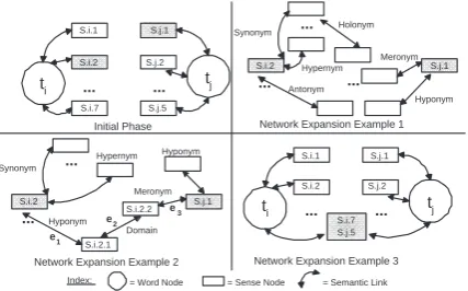
Figure 1: Computation of semantic relatedness.

3.2 Semantic Networks from Word Thesauri

In order to construct a semantic network for a pair of terms t1 andt2 and a combination of their

re-spective senses, i.e., s1 and s2, we adopted the

network construction method that we introduced in (Tsatsaronis et al., 2007). This method was pre-ferred against other related methods, like the one introduced in (Mihalcea et al., 2004), since it em-beds all the available semantic information exist-ing in WordNet, even edges that cross POS, thus offering a richer semantic representation. Accord-ing to the adopted semantic network construction model, each semantic edge type is given a different weight. The intuition behind edge types’ weight-ing is that certain types provide stronger semantic connections than others. The frequency of occur-rence of the different edge types in Wordnet 2.0, is used to define the edge types’ weights (e.g. 0.57

for hypernym/hyponym edges, 0.14 for nominal-ization edges etc.).

Figure 1 shows the construction of a semantic network for two terms ti and tj. Let the

high-lighted senses S.i.2 andS.j.1 be a pair of senses of ti and tj respectively. All the semantic links

of the highlighted senses, as found in WordNet, are added as shown in example 1 of figure 1. The process is repeated recursively until at least one path betweenS.i.2andS.j.1is found. It might be the case that there is no path from S.i.2 toS.j.1. In that case SR((ti, tj),(S.i.2, S.j.1), O) = 0.

Suppose that a path is that of example 2, where

e1, e2, e3are the respective edge weights,d1is the

depth ofS.i.2,d2the depth ofS.i.2.1,d3the depth

ofS.i.2.2andd4 the depth ofS.j.1, anddmax the

maximum thesaurus depth. For reasons of sim-plicity, let e1 = e2 = e3 = 0.5, and d1 = 3.

Naturally,d2 = 4, and letd3 =d4 =d2 = 4.

Fi-nally, letdmax = 14, which is the case for

Word-Net 2.0. Then, SR((ti, tj),(S.i.2, S.j.1), O) =

0.53 ·0.4615 ·0.52 = 0.01442. Example 3 of figure 2 illustrates another possibility whereS.i.7

andS.j.5is another examined pair of senses forti

andtjrespectively. In this case, the two senses

co-incide, andSR((ti, tj),(S.i.7, S.j.5), O) = 1·₁₄d,

wheredthe depth of the sense. When two senses coincide,SCM = 1, as mentioned in definition 1, a secondary criterion must be levied to distinguish the relatedness of senses that match. This crite-rion in SR isSP E, which assumes that a sense is more specific as we traverse WordNet graph downwards. In the specified example,SCM = 1, butSP E= ₁₄d. This will give a final value toSR

that will be less than1. This constitutes an intrin-sic property ofSR, which is expressed bySP E. The rationale behind the computation of SP E

stems from the fact that word senses in WordNet are organized into synonym sets, named synsets. Moreover, synsets belong to hierarchies (i.e., noun hierarchies developed by the hypernym/hyponym relations). Thus, in case two words map into the same synset (i.e., their senses belong to the same synset), the computation of their semantic related-ness must additionally take into account the depth of that synset in WordNet.

3.3 Computing Maximum Semantic Relatedness

In the expansion of the VSM model we need to weigh the inner product between any two term vectors with their semantic relatedness. It is obvi-ous that given a word thesaurus, there can be more than one semantic paths that link two senses. In these cases, we decide to use the path that max-imizes the semantic relatedness (the product of SCM and SPE). This computation can be done according to the following algorithm, which is a modification of Dijkstra’s algorithm for finding the shortest path between two nodes in a weighted directed graph. The proof of the algorithm’s cor-rectness follows with theorem 1.

Theorem 1 Given a word thesaurusO, a weight-ing functionw:E→(0,1), where a higher value declares a stronger edge, and a pair of senses

S(ss, sf) declaring source (ss) and destination

(sf) vertices, then theSCM(S, O)·SP E(S, O)

is maximized for the path returned by Algorithm 1, by using the weighting scheme eij = wij ·

2·di·dj

dmax·(di+dj), whereeij the new weight of the edge

Algorithm 1 MaxSR(G,u,v,w)

Require: A directed weighted graph G, two

nodes u, v and a weighting schemew :E →

(0..1).

Ensure: The path from u to v with the maximum

product of the edges weights.

Initialize-Single-Source(G,u)

1: for all verticesv∈V[G]do 2: d[v] =−∞

3: π[v] =N U LL

4: end for 5: d[u] = 1

Relax(u, v, w)

6: ifd[v]< d[u]·w(u, v)then 7: d[v] =d[u]·w(u, v) 8: π[v] =u

9: end if

Maximum-Relatedness(G,u,v,w)

10: Initialize-Single-Source(G,u)

11: S =∅ 12: Q=V[G] 13: whilev∈Qdo

14: s= Extract fromQthe vertex with maxd 15: S =S∪s

16: for all verticesk∈Adjacency List ofsdo 17: Relax(s,k,w)

18: end for 19: end while

20: return the path following all the ancestorsπof

vback tou

weight assigned by weighting functionw.

Proof 1 For the proof of this theorem we follow

the course of thinking of the proof of theorem

25.10 in (Cormen et al., 1990). We shall show that for each vertex sf ∈ V, d[sf] is the

max-imum product of edges’ weight through the se-lected path, starting from ss, at the time when

sf is inserted into S. From now on, the

nota-tion δ(ss, sf) will represent this product. Path

p connects a vertex in S, namely ss, to a

ver-tex in V −S, namelysf. Consider the first

ver-texsy along p such thatsy ∈ V −S and let sx

be y’s predecessor. Now, path p can be decom-posed as ss → sx → sy → sf. We claim that

d[sy] =δ(ss, sy)whensf is inserted intoS.

Ob-serve thatsx ∈ S. Then, becausesf is chosen as

the first vertex for whichd[sf]6=δ(ss, sf)when it

is inserted intoS, we hadd[sx] =δ(ss, sx)when

sxwas inserted intoS.

We can now obtain a contradiction to the

above to prove the theorem. Because sy

oc-curs before sf on the path fromss to sf and all

edge weights are nonnegative2 and in (0,1) we have δ(ss, sy) ≥ δ(ss, sf), and thus d[sy] =

δ(ss, sy) ≥ δ(ss, sf) ≥ d[sf]. But both sy

and sf were in V − S when sf was chosen,

so we have d[sf] ≥ d[sy]. Thus, d[sy] =

δ(ss, sy) = δ(ss, sf) = d[sf]. Consequently,

d[sf] =δ(ss, sf)which contradicts our choice of

sf. We conclude that at the time each vertexsf is

inserted intoS,d[sf] =δ(ss, sf).

Next, to prove that the returned maximum product is the SCM(S, O) · SP E(S, O), let the path between ss and sf with the maximum

edge weight product have k edges. Then, Al-gorithm 1 returns the maximum Qk

i=1ei(i+1) =

ws2· _dmax2·ds·d2

·(ds+d2) ·w23·

2·d2·d3

dmax·(d2+d3) ·...·wkf ·

2·dk·df

dmax·(dk+df) =

Qk

i=1wi(i+1) · Qki=1 2didi+1 di+di+1 ·

1

dmax =SCM(S, O)·SP E(S, O).

3.4 Word Sense Disambiguation

The reader will have noticed that our model com-putes the SR between two termsti,tj, based on the

pair of sensessi,sj of the two terms respectively,

which maximizes the product SCM ·SP E. Al-ternatively, a WSD algorithm could have disam-biguated the two terms, given the text fragments where the two terms occurred. Though interesting, this prospect is neither addressed, nor examined in this work. Still, it is in our next plans and part of our future work to embed in our model some of the interesting WSD approaches, like knowledge-based (Sinha and Mihalcea, 2007; Brody et al., 2006), corpus-based (Mihalcea and Csomai, 2005; McCarthy et al., 2004), or combinations with very high accuracy (Montoyo et al., 2005).

3.5 The GVSM Model

In equation 2, which captures the document-query similarity in the GVSM model, the orthogonality between termsti andtj is expressed by the inner

product of the respective term vectorst~it~j. Recall

that~tiandt~j are in reality unknown. We estimate

their inner product by equation 3, where si and

sj are the senses of terms ti and tj respectively,

maximizingSCM ·SP E.

~

tit~j =SR((ti, tj),(si, sj), O) (3)

Since in our model we assume that each term can be semantically related with any other term, and

SR((ti, tj), O) = SR((tj, ti), O), the new space

is of n·(n−1)

2 dimensions. In this space, each

di-mension stands for a distinct pair of terms. Given a document vectord~kin the VSM TF-IDF space,

we define the value in the (i, j) dimension of the new document vector space as dk(ti, tj) =

(T F −IDF(ti, dk) +T F −IDF(tj, dk))·~tit~j.

We add the TF-IDF values because any product-based value results to zero, unless both terms are present in the document. The dimensionsq(ti, tj)

of the query, are computed similarly. A GVSM model aims at being able to retrieve documents that not necessarily contain exact matches of the query terms, and this is its great advantage. This new space leads to a new GVSM model, which is a natural extension of the standard VSM. The co-sine similarity between a documentdkand a query

qnow becomes:

cos(_d~_{k, ~}q) =

Pn i=1

Pn

j=idk(ti, tj)·q(ti, tj)

q Pn

i=1

Pn

j=idk(ti, tj)2·

q Pn

i=1

Pn

j=iq(ti, tj)2

(4)

wherenis the dimension of the VSM TF-IDF space.

4 Experimental Evaluation

The experimental evaluation in this work is two-fold. First, we test the performance of the seman-tic relatedness measure (SR) for a pair of words in three benchmark data sets, namely the Ruben-stein and Goodenough 65 word pairs (Ruben-stein and Goodenough, 1965)(R&G), the Miller and Charles 30 word pairs (Miller and Charles, 1991)(M&C), and the 353 similarity data set (Finkelstein et al., 2002). Second, we evaluate the performance of the proposed GVSM in three TREC collections (TREC 1, 4 and 6).

4.1 Evaluation of the Semantic Relatedness Measure

For the evaluation of the proposed semantic re-latedness measure between two terms we experi-mented in three widely used data sets in which hu-man subjects have provided scores of relatedness for each pair. A kind of ”gold standard” ranking of related word pairs (i.e., from the most related words to the most irrelevant) has thus been cre-ated, against which computer programs can test their ability on measuring semantic relatedness be-tween words. We compared our measure against ten known measures of semantic relatedness: (HS) Hirst and St-Onge (1998), (JC) Jiang and Conrath (1997), (LC) Leacock et al. (1998), (L) Lin (1998), (R) Resnik (1995), (JS) Jarmasz and Szpakowicz

(2003), (GM) Gabrilovich and Markovitch (2007), (F) Finkelstein et al. (2002), (HR) ) and (SP) Strube and Ponzetto (2006). In Table 1 the results of SR and the ten compared measures are shown. The reported numbers are the Spearman correla-tion of the measures’ rankings with the gold stan-dard (human judgements).

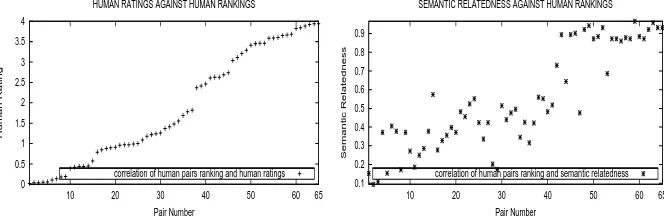
The correlations for the three data sets show that SR performs better than any other measure of se-mantic relatedness, besides the case of (HR) in the M&C data set. It surpasses HR though in the R&G and the 353-C data set. The latter contains the word pairs of the M&C data set. To visualize the performance of our measure in a more comprehen-sible manner, Figure 2 presents for all pairs in the R&G data set, and with increasing order of relat-edness values based on human judgements, the re-spective values of these pairs that SR produces. A closer look on Figure 2 reveals that the values pro-duced by SR (right figure) follow a pattern similar to that of the human ratings (left figure). Note that the x-axis in both charts begins from the least re-lated pair of terms, according to humans, and goes up to the most related pair of terms. The y-axis in the left chart is the respective humans’ rating for each pair of terms. The right figure shows SR for each pair. The reader can consult Budanitsky and Hirst (2006) to confirm that all the other mea-sures of semantic relatedness we compare to, do not follow the same pattern as the human ratings, as closely as our measure of relatedness does (low y values for small x values and high y values for high x). The same pattern applies in the M&C and 353-C data sets.

4.2 Evaluation of the GVSM

For the evaluation of the proposed GVSM model, we have experimented with three TREC collec-tions 3, namely TREC 1 (TIPSTER disks 1 and 2), TREC 4 (TIPSTER disks 2 and 3) and TREC 6 (TIPSTER disks 4 and 5). We selected those TREC collections in order to cover as many dif-ferent thematic subjects as possible. For example, TREC 1 contains documents from the Wall Street Journal, Associated Press, Federal Register, and abstracts of U.S. department of energy. TREC 6 differs from TREC 1, since it has documents from Financial Times, Los Angeles Times and the For-eign Broadcast Information Service.

For each TREC, we executed the standard

HS JC LC L R JS GM F HR SP SR

R&G 0.745 0.709 0.785 0.77 0.748 0.842 0.816 N/A 0.817 0.56 0.861

M&C 0.653 0.805 0.748 0.767 0.737 0.832 0.723 N/A 0.904 0.49 0.855

353-C N/A N/A 0.34 N/A 0.35 0.55 0.75 0.56 0.552 0.48 0.61

Table 1: Correlations of semantic relatedness measures with human judgements.

0 0.5 1 1.5 2 2.5 3 3.5 4

10 20 30 40 50 60 65

Human Rating

Pair Number HUMAN RATINGS AGAINST HUMAN RANKINGS

correlation of human pairs ranking and human ratings

0.1 0.2 0.3 0.4 0.5 0.6 0.7 0.8 0.9

10 20 30 40 50 60 65

Semantic Relatedness

Pair Number

SEMANTIC RELATEDNESS AGAINST HUMAN RANKINGS

correlation of human pairs ranking and semantic relatedness

Figure 2: Correlation between human ratings and SR in the R&G data set.

line TF-IDF VSM model for the first 20 topics of each collection. Limited resources prohibited us from executing experiments in the top 1000

documents. To minimize the execution time, we have indexed all the pairwise semantic related-ness values according to the SR measure, in a database, whose size reached 300GB. Thus, the execution of the SR itself is really fast, as all pair-wise SR values between WordNet synsets are in-dexed. For TREC 1, we used topics51−70, for TREC 4 topics201−220and for TREC 6 topics

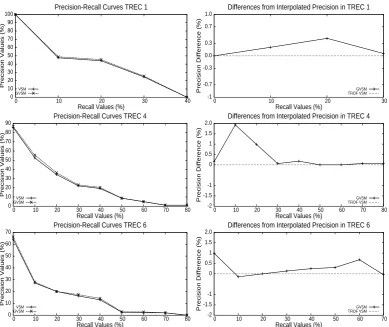
301−320. From the results of the VSM model, we kept the top-50 retrieved documents. In order to evaluate whether the proposed GVSM can aid the VSM performance, we executed the GVSM in the same retrieved documents. The interpo-lated precision-recall values in the 11-standard re-call points for these executions are shown in fig-ure 3 (left graphs), for both VSM and GVSM. In the right graphs of figure 3, the differences in in-terpolated precision for the same recall levels are depicted. For reasons of simplicity, we have ex-cluded the recall values in the right graphs, above which, both systems had zero precision. Thus, for TREC 1 in the y-axis we have depicted the differ-ence in the interpolated precision values (%) of the GVSM from the VSM, for the first4recall points. For TRECs 4 and 6 we have done the same for the first9and8recall points respectively.

As shown in figure 3, the proposed GVSM may improve the performance of the TFIDF VSM up to

1.93%in TREC 4,0.99%in TREC 6 and0.42%

in TREC 1. This small boost in performance proves that the proposed GVSM model is promis-ing. There are many aspects though in the GVSM that we think require further investigation, like for example the fact that we have not conducted WSD so as to map each document and query term oc-currence into its correct sense, or the fact that the weighting scheme of the edges used in SR gen-erates from the distribution of each edge type in WordNet, while there might be other more sophis-ticated ways to compute edge weights. We believe that if these, but also more aspects discussed in the next section, are tackled, the proposed GVSM may improve more the retrieval performance.

5 Future Work

0 10 20 30 40 50 60 70 80 90 100

0 10 20 30 40

Precision Values (%)

Recall Values (%)

Precision-Recall Curves TREC 1

VSM GVSM

-1 -0.7 -0.3 0.0 0.3 0.7 1.0

0 10 20 30

Precision Difference (%)

Recall Values (%)

Differences from Interpolated Precision in TREC 1

GVSM TFIDF VSM

0 10 20 30 40 50 60 70 80 90

0 10 20 30 40 50 60 70 80

Precision Values (%)

Recall Values (%)

Precision-Recall Curves TREC 4

VSM GVSM

-2 -1.5 -1 0 0.5 1 1.5 2.0

0 10 20 30 40 50 60 70 80

Precision Difference (%)

Recall Values (%)

Differences from Interpolated Precision in TREC 4

GVSM TFIDF VSM

0 10 20 30 40 50 60 70

0 10 20 30 40 50 60 70 80

Precision Values (%)

Recall Values (%)

Precision-Recall Curves TREC 6

VSM GVSM

-2 -1.5 -1 0 0.5 1 1.5 2.0

0 10 20 30 40 50 60 70

Precision Difference (%)

Recall Values (%)

Differences from Interpolated Precision in TREC 6

GVSM TFIDF VSM

Figure 3: Differences (%) from the baseline in interpolated precision.

added into the model. Since we are using a large knowledge-base (WordNet), we can add a simple method to look-up term occurrences in a specified window and check whether they form a phrase. This would also decrease the ambiguity of the re-spective text fragment, since in WordNet a phrase is usually monosemous.

Moreover, there are additional aspects that de-serve further research. In previously proposed GVSM, like the one proposed by Voorhees (1993), or by Mavroeidis et al. (2005), it is suggested that semantic information can create an individual space, leading to a dual representation of each doc-ument, namely, a vector with document’s terms and another with semantic information. Ratio-nally, the proposed GVSM could act complemen-tary to the standard VSM representation. Thus, the similarity between a query and a document may be computed by weighting the similarity in the terms space and the senses’ space. Finally, we should also examine the perspective of applying the pro-posed measure of semantic relatedness in a query expansion technique, similarly to the work of Fang (2008).

6 Conclusions

References

R. Baeza-Yates and B. Ribeiro-Neto. 1999. Modern

Information Retrieval. Addison Wesley.

S. Brody, R. Navigli, and M. Lapata. 2006. Ensemble methods for unsupervised wsd. In Proc. of

COL-ING/ACL 2006, pages 97–104.

A. Budanitsky and G. Hirst. 2006. Evaluating

wordnet-based measures of lexical semantic related-ness. Computational Linguistics, 32(1):13–47.

T.H. Cormen, C.E. Leiserson, and R.L. Rivest. 1990.

Introduction to Algorithms. The MIT Press.

H. Fang. 2008. A re-examination of query expansion using lexical resources. In Proc. of ACL 2008, pages 139–147.

C. Fellbaum. 1998. WordNet – an electronic lexical

database. MIT Press.

L. Finkelstein, E. Gabrilovich, Y. Matias, E. Rivlin, Z. Solan, G. Wolfman, and E. Ruppin. 2002. Plac-ing search in context: The concept revisited. ACM

TOIS, 20(1):116–131.

E. Gabrilovich and S. Markovitch. 2007. Computing semantic relatedness using wikipedia-based explicit semantic analysis. In Proc. of the 20th IJCAI, pages 1606–1611. Hyderabad, India.

G. Hirst and D. St-Onge. 1998. Lexical chains as rep-resentations of context for the detection and correc-tion of malapropisms. In WordNet: An Electronic

Lexical Database, chapter 13, pages 305–332,

Cam-bridge. The MIT Press.

M. Jarmasz and S. Szpakowicz. 2003. Roget’s the-saurus and semantic similarity. In Proc. of

Confer-ence on Recent Advances in Natural Language Pro-cessing, pages 212–219.

J.J. Jiang and D.W. Conrath. 1997. Semantic similarity based on corpus statistics and lexical taxonomy. In

Proc. of ROCLING X, pages 19–33.

R. Krovetz and W.B. Croft. 1992. Lexical ambigu-ity and information retrieval. ACM Transactions on

Information Systems, 10(2):115–141.

C. Leacock, G. Miller, and M. Chodorow. 1998.

Using corpus statistics and wordnet relations for

sense identification. Computational Linguistics,

24(1):147–165, March.

D. Lin. 1998. An information-theoretic definition of similarity. In Proc. of the 15th International

Con-ference on Machine Learning, pages 296–304.

D. Mavroeidis, G. Tsatsaronis, M. Vazirgiannis, M. Theobald, and G. Weikum. 2005. Word sense disambiguation for exploiting hierarchical thesauri

in text classification. In Proc. of the 9th PKDD,

pages 181–192.

D. McCarthy, R. Koeling, J. Weeds, and J. Carroll. 2004. Finding predominant word senses in untagged

text. In Proc, of the 42nd ACL, pages 280–287.

Spain.

R. Mihalcea and A. Csomai. 2005. Senselearner:

Word sense disambiguation for all words in unre-stricted text. In Proc. of the 43rd ACL, pages 53–56.

R. Mihalcea, P. Tarau, and E. Figa. 2004. Pagerank on semantic networks with application to word sense disambiguation. In Proc. of the 20th COLING.

G.A. Miller and W.G. Charles. 1991. Contextual cor-relates of semantic similarity. Language and

Cogni-tive Processes, 6(1):1–28.

A. Montoyo, A. Suarez, G. Rigau, and M. Palomar.

2005. Combining knowledge- and corpus-based

word-sense-disambiguation methods. Journal of

Ar-tificial Intelligence Research, 23:299–330, March.

P. Resnik. 1995. Using information content to evalu-ate semantic similarity. In Proc. of the 14th IJCAI, pages 448–453, Canada.

H. Rubenstein and J.B. Goodenough. 1965. Contex-tual correlates of synonymy. Communications of the

ACM, 8(10):627–633.

G. Salton and M.J. McGill. 1983. Introduction to

Modern Information Retrieval. McGraw-Hill.

M. Sanderson. 1994. Word sense disambiguation and information retrieval. In Proc. of the 17th SIGIR, pages 142–151, Ireland. ACM.

R. Sinha and R. Mihalcea. 2007. Unsupervised graph-based word sense disambiguation using measures of word semantic similarity. In Proc. of the IEEE

In-ternational Conference on Semantic Computing.

C. Stokoe, M.P. Oakes, and J. Tait. 2003. Word sense disambiguation in information retrieval revisited. In

Proc. of the 26th SIGIR, pages 159–166.

M. Strube and S.P. Ponzetto. 2006. Wikirelate!

com-puting semantic relatedness using wikipedia. In

Proc. of the 21st AAAI.

G. Tsatsaronis, M. Vazirgiannis, and I. Androutsopou-los. 2007. Word sense disambiguation with spread-ing activation networks generated from thesauri. In

Proc. of the 20th IJCAI, pages 1725–1730.

E. Voorhees. 1993. Using wordnet to disambiguate word sense for text retrieval. In Proc. of the 16th

SIGIR, pages 171–180. ACM.

S.K.M. Wong, W. Ziarko, V.V. Raghavan, and P.C.N. Wong. 1987. On modeling of information retrieval concepts in vector spaces. ACM Transactions on