The linear Monge Kantorovitch linear colour mapping for example based colour transfer

The Linear Monge-Kantorovitch Linear Colour Mapping for

Example-Based Colour Transfer.

F. Piti´e, A. Kokaram

Sigmedia.tv,

Trinity College Dublin, Ireland, [email protected]

Keywords: Colour Transfer, Colour Grading, Monge-Kantorovitch.

Abstract

A common task in image editing is to change the colours of a picture to match the desired colour grade of another picture. Finding the correct colour mapping is tricky because it involves numerous interrelated operations, like balancing the colours, mixing the colour channels or adjusting the contrast. Recently, a number of automated tools have been proposed to find an adequate one-to-one colour mapping. The focus in this paper is on finding the best linear colour transformation. Linear transformations have been proposed in the literature but independently. The aim of this paper is thus to establish a common mathematical background to all these methods. Also, this paper proposes a novel transformation, which is derived from the Monge-Kantorovicth theory of mass transportation. The proposed solution is optimal in the sense that it minimises the amount of changes in the picture colours. It favourably compares theoretically and experimentally with other techniques for various images and under various colour spaces.

1 Introduction

Adjusting the colour grade of pictures is an important step in professional photography and in the movie post-production. This process is part of the larger activity of grading in which the colour and grain aspects of the photographic material are digitally manipulated. In particular, a main problem in the movie industry is to adjust the colour consistently across all the shots, even though the movie has been edited with heterogeneous video material. Shots taken at different times under natural light can have a substantially differentfeeldue to even slight changes in lighting. Colour grading is a delicate task since the slightest of colour variations can alter the mood of a picture.

Typical tuning operations comprise adjusting the exposure, brightness and contrast, calibrating the white point or finding a colour mapping curve for the luminance levels and the three colour channels. For instance, in an effort to balance the contrast of the red colour, the digital samples in the red channel in one frame may be multiplied by some gain factor and the output image viewed and compared to the colour of some

other (a target) frame. The gain is then adjusted if the match in colour is not quite right. The amount of adjustment and whether it is an increase or decrease depends crucially on the experience of the artist. An another problem is that most of these operations are interdependent. For instance, the contrast on the red channel can change after a mixing of the colour channels. It would be therefore beneficial to automate this task in some way.

This paper presents techniques which aim at facilitating the choice of the colour mappings. These techniques belong to the class of example-based colour transfer methods. The idea, first formulated by Reinhardet al.[13], has raised a lot of interest recently [1, 8, 19, 11]. Figure 1 illustrates this with an example. The original picture (a) is transformed so that its colours match the palette of the image (b), regardless of the content of the pictures. Consider the two pictures as two sets of three dimensional colour pixels. A way of treating the re-colouring problem would be to find a one-to-one colour mapping that is applied for every pixel in the original image. For example in Figure 1, every blue pixel is re-coloured in green. The new picture is identical in every aspect to the original picture, except that the picture now exhibits the same colour statistics, or palette, as the target picture.

Employing a one-to-one colour mapping is a standard method in the industry, but note that more complicated grading techniques based on local manipulations have also been proposed [16],[3],[20]. These techniques will not be discussed here but a comprehensive review can be found in [12].

(a) Original (b) Target Colour Palette (c) Result

Figure 1: Colour transfer example. A colour mapping is applied on the original picture (a) to match the palette of an example (b) provided by the user.

combine the following 6 adjustment functions: “levels”, “brightness/contrast”, “color balance”, “Hue/Saturation”, “Channel Mixer” and “Photo Filter”. Finding automatically the linear transformation would save a lot of time.

Linear colour transfer techniques actually exist in the literature. In particular Abadpour and Kasaei [1] and Kotera [19] have presented simple solutions to this problem. In fact it transpires from the literature that numerous linear transformations can achieve an exact transfer of the statistics. The first contribution of this paper is to mathematically characterise the ensemble of these linear transformations. This gives a common mathematical background to these methods. The second contribution of this paper is to introduce a new transformation which is based on the Monge-Kantorovitch (MK) of mass transportation. This solution is optimal in the sense that it minimises the amount of colour changes. This MK transformation turns out to be very intuitive from an artist point of view because it has monotonous properties. For instance the brightest and the darkest points remains the brightest and darkest points after transformation. It is also shown here that the MK transformation is independent to orthogonal colour space conversions.

Organisation of the Paper. The problem is first formalised in section 2. The ensemble of the all possible linear transformations is then characterised in section 3. The review of existing techniques is then presented in section 4. The review is accompanied with a table of comparative results. The optimal Monge-Kantorovitch solution is then presented in section 5. The last section 6 examines the influence on the Monge-Kantorovitch transformation when working under different colour-spaces.

2 Mathematical Background of Linear Colour Distribution Transfer

The notion of colour statistics can be understood if an image is represented as a set of colour samples. When working in RGB colour space, the image is then represented by the set of the RGB colour samples(R(i)_{, G}(i)_{, B}(i)₎

1≤i≤M. In a

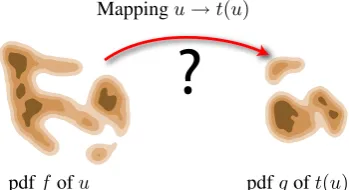
Mappingu→t(u)

?

pdffofu pdfgoft(u)

Figure 2: Distribution Transfer Concept. How to find a mapping that transforms the distribution on the left to the distribution on the right?

probabilistic sense, these colour samples are realisations of a 3-dimensional colour random variable and which will be denoted asufor the original image andvfor the target palette image. The colour palette of the original and target pictures correspond then to the distributions ofuandv.

To simplify the presentation of the problem, it is supposed here that both distributions have absolutely continuous probability density function (pdf)f andg. The problem of colour transfer is to find aC1 _{continuous mappingu → t(u), such that the}

new colour distribution oft(u)matches the target distribution

g. This latter problem, illustrated in Figure 2 is also known as the mass preserving transport problem in the mathematic literature[4, 5, 18].

The mapping is in essence a change of variables. Thus the transfer equation can be written as:

f(u)du=g(v)dv ⇒ f(u) =g(t(u))|detJt(u)| (1) whereJt(u) is the Jacobian of t taken atu. The constraint is very complicated in the general case, but in this paper, the problem is restricted to linear mappings. Mappings are then of the formt(u) =T u+t0whereTis aN×N matrix (width

N = 3for colour). In that form, the Jacobian is thenJt(u) =T and the quantity|detJt(u)|=|detT|is also constant, thus

general case, but, as it shown hereafter, this can always be achieved when both the original distributionsf and the target distributionsgare multivariate Gaussian distributions (MVG) denoted asN(µu,Σu)andN(µv,Σv):

f(u)∝exp

−1

2(u−µu)

T_Σ−1

u (u−µu)

g(v)∝exp

−1

2(v−µv)

T_Σ−1

v (v−µv)

(3)

withΣuandΣvthe covariance matrices ofuandv. Note that when the distributions are not MVG, a MVG approximation can always be obtained by estimating the mean and the covariance matrices of the distributions. To have the pdf transfer condition of equation (2),i.e.g(t(u))∝f(u), it must hold that:

(t(u)−µv)TΣ−1v (t(u)−µv) = (u−µu)TΣ−1u (u−µu) (4) Thustmust satisfyt(u) =T(u−µu) +µvwithTTΣ−1v T =

Σ−1_u , or equivalentlyTΣuTT = Σu:

(

t(u) =T(u−µu) +µv

TΣuTT = Σv

(5)

It turns out that there are numerous solutions for the matrixT

and thus multiple ways of transferring the colour statistics.

3 Characterisation of the Transformations

The main reason why there is more than one solution is because the covariance matricesΣuandΣvadmit more than one square root,i.e. that there is more than one square matrixAsuch that

Σu=AAT. To understand this, consider two particular square rootsAandB such that Σu = AAT andΣv = BBT. For instance the square roots can be found by taking the Cholesky decomposition: A = chol(Σu)and B = chol(Σv). In this case both A and B are lower triangle matrices. Consider then the development of equation (5):

TΣuTT = Σv (6)

T AAT

TT = BBT (7)

(T A) (T A)T = BBT (8)

One solution forTwill be to setT A=Band takeT =BA−1

as a solution. However this is not the only solution. Observe that bothT A andB are square roots ofΣv. An interesting result about matrices square root, is that all square roots of a positive matrix are related by orthogonal transformations. This means here that there exists an orthogonal matrixQthat links

T AtoBby:

T A=BQ (9) Rearranging this equation yields to the complete characterisation of the solutions. Any valid transformation can thus be derived from two given square root matricesAandB

ofΣuandΣvby:

T =BQA−1withQTQ=Id (10)

Thus all the following solutions in this paper only differ for the choice of this inner orthogonal matrixQ. This choice yields however to very different properties for the transformations.

4 Review of Existing Linear Transfers

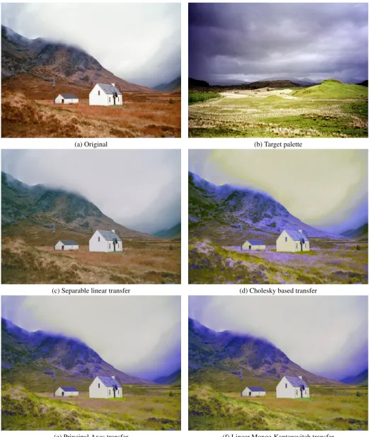
This section presents some particular transformations that have been explored in the colour grading literature. The different techniques are compared to each other on a practical example in Figure 3. The original image is depicted in Figure 3-a and the target palette is displayed in Figure 3-b. All colour transfers are done in the RGB space. Note that further comparison analysis for different colour spaces is carried out in section 6.

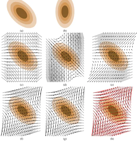
In addition to the comparison on this colour transfer example, it would be interesting to visualise the geometrical differences between the colour mappings. This is presented in Figure 4, which shows some the mappings for a 2D case. The original MVG f is displayed Figure 4-a, and the target MVG g is displayed on Figure 4-b. Figure 4-c to Figure 4-g overlay the estimated 2D transformation on the original distribution.

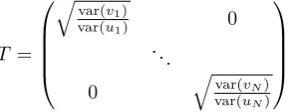
4.1 Independent Transfer

The first linear method, used by Reinhard et al.[14] in their original paper on colour transfer, is to simply match the means and the variances of each component independently. This transformation is not a limited solution as it assumes that both distributions are separable. The covariance matrices are assumed to be diagonal: Σu = diag(var(u1), . . . ,var(uN)) and Σv = diag(var(v1), . . . ,var(vN)). It yields for the mapping that T=     

q_var(v

1)

var(u1) 0

. ._.

0

q var(vN) var(uN)

     (11)

The independence assumption is simplistic and is rarely valid for real images. The poor quality of the transfer in the results in Figure 3-c shows that this is indeed not always the case. The solution proposed by Reinhard is to work in the decorrelated colour spacelαβof Ruderman [15]. This helps to some extent but cannot guarantee a full decorrelation between components.

4.2 Cholesky Decomposition

Following the characterisation of section 3, an exact solution can be obtain using the Cholesky decomposition ofΣu =LuLTu andΣv =LvLTv whereLuandLv are lower triangular matrices with strictly positive diagonal elements. This decomposition yields the following solution:

the Cholesky decomposition can lead to radically different transformation if instead of u = (u2, u1) it is considered

u= (u1, u2). This mean for instance that the channel ordering

RGBleads to different results that with the channel ordering

BGR.

4.3 Square Root Decomposition

Another popular solution [10, 6, 1, 2, 17] is to find the mapping that realigns the principal axes of Σv to that of Σu. In this solution the covariances matrices are decomposed into symmetric definite positive matrices. This done by using the square root operator for symmetric positive semidefinite matrices. There are multiple square roots for matrices, but if the matrix is symmetric positive then there is only one symmetric positive square root matrix. Denote as Σ1u/2 and

Σ1v/2these positive square roots. They can be obtained via the spectral decomposition ofΣuandΣv:

Σu=PuTDuPu and Σ1u/2=P T uD

1/2

u Pu (13)

Σv =PvTDvPv and Σ1v/2=P T v D

1/2

v Pv (14) where Pu and Pv are orthogonal matrices and Du and Dv the diagonal matrix containing the (positive) eigenvalues of

Σu and Σv. Since Σ

1/2

u and Σ

1/2

v are uniquely defined, no special arrangement of the eigenvectors is necessary. These decompositions lead to the following mapping:

T = Σ1_v/2Σ−1_u /2 (15)

Results displayed in Figure 3-e show an improvement over the mapping based on the Cholesky decomposition. Note in particular that the violet colour of the grass in Figure 3-e is not present here. This is due to fact that the mapping here does not depend on the channel ordering.

In fact, this paper shows hereafter that this transformation is independent of orthogonal transformations. Consider an orthogonal transformation defined as u → Hu. To be independent under the transformationH, it must be shown that the transformationT is the same up to the transformationH, i.e.thatTHu→Hv =HTTu→vH. To show this, it is sufficient to realise that:

Σ1_Hu/2 = HTΣuH

1/2

(16)

= HTPuTDuPuH

1/2

(17)

sincePuHis also orthogonal, it yields that

Σ1_Hu/2 = HTP_uT(Du)

1/2

PuH (18)

= HT(Σu)1/2H (19)

Thus

THu→Hv = Σ

1/2

HvΣ

−1/2

Hu (20)

= HTΣ1v/2HHTΣ−1u /2H (21)

= HTTu→vH (22)

This property of independence to orthogonal transformations is a major advantage over the Choleski based method. This means that the colour transfer has mainly the same effect under different colour spaces, which is clearly not the case with Choleski.

5 The Linear Monge-Kantorovitch Solution

The problem encountered with most of the presented transformations is that the geometry of the resulting mapping might not be as it was intended. For example, it is not guaranteed that a transfer will not map black pixels to white and conversely white pixels to black. The resulting picture could have the colour proportions as expected, but locally the colours would be swapped. To avoid this problem, a good solution is to further constrain the transfer problem and look for a mapping that also minimise its displacement cost:

I[t] = Z

u

kt(u)−uk2_f(u)du

(23)

Finding this minimal displacement mapping in the general case is known as theMonge’s optimal transportation problem. Monge’s problem has raised a major interest in mathematics in recent years [4, 5, 18] as it has been found to be relevant for many scientific fields like fluid mechanics.

To understand the interest of the MK solution in colour grading, three aspects of the MK solutions will be reported here. The first result of importance is that the MK solution always exists for continuous pdfs and is unique. This means that there is no room left for ambiguity. The second result, which is of interest here, is that the MK solution is the gradient of a convex function1:

t=∇φ where φ:RN →R is convex (24)

This property might seem quite obscure at first sight, but this simply is the equivalent of monotonicity for one dimensional functions inR. It implies for instance that the brightest areas of

a picture still remain the brightest areas after mapping. The MK solution is thus geometrically more intuitive than the Cholesky or the Principal Axes solution. One could be concerned that the MK solution might not be linear for MVG distributions. Fortunately the solution for MVGs is actually linear and admits a simple closed form. The detailed proof of how to find the MK mapping can be found in [9]. The mainstay of the reasoning is that since the MK solution is the gradient of a convex function, the matrixThas to be symmetric definite positive, which leads to this unique solution forT:

T = Σ−1_u /2Σ_u1/2ΣvΣ1u/2

1/2

Σ−1_u /2 (25)

The corresponding results in Figure 3-f are convincing. The results are slightly better than the ones of the Principal Axes method. For instance a pink trace on the grass in front of the

1_{A convex function [5]φ:}

house is visible in (e) but not in (f). The difference between the PCA and the MK mappings can also be seen on Figure 4-f where both mappings have been overlaid.

Note that, like the PCA based transformation, the MK transformation is independent of orthogonal transformations. The MK solution is thus interesting as it provides an intuitive and probably better mapping for a similar computational complexity to the popular methods.

6 Comparisons in different Colour Spaces

If a method can exactly transfer the complete colour statistics, then this method will work regardless of the chosen colour space. Thus, in that respect, the colour space is not important to transfer the colour ‘feel‘ of an image.

The colour space has however an influence on the geometrical form of the colour mapping. It is now known that the PCA and MK transformations are independent to orthogonal transformations, so the influence of the colour space is not as dramatic as it can be for the Choleski method. However these methods are not independent to non-linear colour space transformations or even colour scaling.

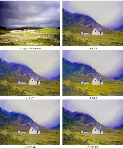
In the MK formulation for instance, the cost of transportation is related to the colour difference, which depends on the chosen colour space. Thus uniform colour spaces like YUV, or better CIELAB and CIELUV, are preferable to the basic RGB to obtain coherent colour mappings. Comparative results for RGB, YUV, CIE XYZ, CIELAB and CIELUV are displayed in Figure 5 for the linear MK solution. Differences might be difficult to see on printed images, but these are very significant when displayed on a big screen, especially if they are images in a sequence which is played back. The CIELAB colour space overall offers better renderings, for the linear and the non-linear case. This is because it is designed to measure the difference between colours under different illuminants.

7 Conclusion

The study conducted in the paper has established a solid background to understand differences in linear colour transformations for example-based colour transfer. The linear Monge-Kantorovicth solution, which is to our knowledge introduced here for the first time in the image processing community, offers a number of advantages over previously proposed transformations. It gives to the user intuitive guarantees on the colour transfer:

1. it minimises the amount of colour changes

2. it has some nice monotonicity property and thus preserves the relative positions of colours

3. it produces relatively similar results under different colour spaces

The linear Monge-Kantorovitch seems therefore to be a good choice in an interactive post-production environment.

Acknowledgements

This work supported by Adobe Inc, SJ, USA. The authors would also like to thanks the people at The Foundry for their remarks and feedback.

References

[1] A. Abadpour and S. Kasaei. A fast and efficient fuzzy color transfer method. In Proceedings of the IEEE Symposium on Signal Processing and Information Technology, pages 491–494, 2004.

[2] A. Abadpour and S. Kasaei. An efficient pca-based color transfer method. Journal of Visual Communication and Image Representation, 18(1):15–34, 2007.

[3] S. Bae, S. Paris, and F. Durand. Two-scale tone management for photographic look. ACM Transactions on Graphics (Proceedings of ACM SIGGRAPH 2006), pages 637–645, 2006.

[4] L. C. Evans. Partial differential equations and Monge-Kantorovich mass transfer. Current Developments in Mathematics, 1997, pages 65–126, 1998.

[5] W. Gangbo and R. McCann. The geometry of optimal transport.Acta Mathematica, pages 113–161, 1996.

[6] H. Kotera. A scene-referred color transfer for pleasant imaging on display. In Proceedings of the IEEE International Conference on Image Processing, pages 5– 8, 2005.

[7] J. Morovic and P-L. Sun. Accurate 3d image colour histogram transformation. Pattern Recognition Letters, 24(11):1725–1735, 2003.

[8] L. Neumann and A. Neumann. Color style transfer techniques using hue, lightness and saturation histogram matching. In Proceedings of Computational Aestetics in Graphics, Visualization and Imaging, pages 111–122, 2005.

[9] I Olkin and F. Pukelsheim. The distance between two random vectors with given dispersion matrices. Linear Algebra and its Applications, 48:257–263, 1982.

[10] F. Piti´e. Statistical Signal Processing Techniques for Visual Post-Production. PhD thesis, University of Dublin, Trinity College, April 2006.

[11] F. Piti´e, A. Kokaram, and R. Dahyot. N-Dimensional Probability Density Function Transfer and its Application to Colour Transfer. In International Conference on Computer Vision (ICCV’05), Beijing, October 2005.

(a) Original (b) Target palette

(c) Separable linear transfer (d) Cholesky based transfer

(e) Principal Axes transfer (f) Linear Monge-Kantorovitch transfer

(a) (b)

(c) (d) (e)

(f) (g) (h)

(a) target colour palette (b) RGB

(c) YUV (d) XYZ

(e) CIELAB (f) CIELUV

[13] E. Reinhard, M. Ashikhmin, B. Gooch, and P. Shirley. Color transfer between images.IEEE Computer Graphics Applications, 21(5):34–41, 2001.

[14] E. Reinhard, M. Stark, P. Shirley, and J. Ferwerda. Photographic tone reproduction for digital images. ACM Transactions on Graphics, 21(3):267–276, 2002.

[15] D. L. Ruderman, T. W. Cronin, and C. C. Chiao. Statistics of Cone Responses to Natural Images: Implications for Visual Coding.Journal of the Optical Society of America, (8):2036–2045, 1998.

[16] H. L. Shen and J. H. Xin. Transferring color between three-dimensional objects. Applied Optics, 44(10):1969– 1976, April 2005.

[17] H. J. Trussell and M. J. Vrhel. Color correction using principle components. In M. R. Civanlar, S. K. Mitra, and R. J. Moorhead, II, editors,Proc. of Society of Photo-Optical Instrumentation Engineers (SPIE), volume 1452, pages 2–9, June 1991.

[18] C. Villani. Topics in Optimal Transportation, volume 58 of Graduate Studies in Mathematics. American Mathematical Society, Providence, RI, 2003.

[19] C. M. Wang and Y. H. Huang. A novel color transfer algorithm for image sequences. Journal of Information Science and Engineering, 20(6):1039–1056, November 2004.