Consideration on Sensitivity for
Multiple Correspondence Analysis
Masaaki Ida
∗Abstract– Correspondence analysis is a popular re-search technique applicable to data and text mining, because the technique can analyze simple and mul-tiple cross tables containing some measure of corre-spondence between the rows and columns and also has the strength of graphical display in two or three dimensions. The results of correspondence analysis provide information similar to factor analysis. Those abilities will deepen the global understanding on the characteristics of accumulated numerical and text in-formation and have possibility leads to new knowledge discovery. We have so far focused on the text infor-mation of Japanese higher education institution such as syllabuses. We conducted research on collecting and analyzing the information, and on text mining to analyze and visualize the information for grasp-ing the global characteristics of curricula of univer-sities. Moreover, we have considered the sensitivity of ordinary simple correspondence analysis in case of data perturbation. However, more considerations on multiple correspondence analysis are required. This article presents mathematical considerations on sen-sitivity of multiple correspondence analysis.
Keywords: Multiple correspondence analysis, sensitiv-ity analysis, visualization, text mining
1
Introduction
Correspondence analysis is a method to analyze corre-sponding relation between data in multiple categories ex-pressed by cross table. Correspondence analysis is fre-quently utilized for visualization in text mining. Vari-ous comprehensive considerations on overall accumulated data can be taken by executing the correspondence ysis. This method is closely related to homogeneity anal-ysis, dual scaling, and quantification methods.
In a practical situation, elements of the cross table, num-bers of elements, include uncertain information. There-fore, it is necessary to examine perturbations of the result of correspondence analysis.
This paper presents an extension of our former studies for sensitivity of simple correspondence analysis to multiple
correspondence analysis. Section two shows an
exam-∗National Institution for Academic Degrees and University
Evaluation, Gakuen-Nishimachi Kodaira, Tokyo, 187-8587 Japan. Email: [email protected]
ple of comparative analysis for curricula of some higher education institutions with data perturbation. Section three presents mathematical consideration on sensitivity ofmultiplecorrespondence analysis,
2
Comparative Analysis of Curricula
2.1
Syllabus Sets and Cross Table
We developed the curriculum analysis system based on clustering and correspondence analysis for syllabus data, which is applied for some departments of Japanese uni-versities [1, 2, 3, 4].
Procedure of the analysis system is simply described as follows: (1) Collection of curriculum information or syl-labuses. (2) Categorizing (clustering) based on the tech-nical terms in contents of syllabuses. (3) Visualization for the distribution of syllabus or technical term cate-gories and curricula by using correspondence analysis.
As an example [4], we choose five departments or five universities whose department name include media in Japanese from Japanese universities. These department names including mediaare listed in Table 1.
Table 1: Departments offive universities: “media” Univ. Name of department
U1 Department of Media Technology
U2 Department of Media and Image Technology U3 Department of Multimedia Studies
U4 Department of Media Arts, Science and Technology U5 Department of Social and Media Studies
In the categorizing procedure (2), we use the library clas-sification system, NDC: Nippon Decimal Classification
[5]. This system is based on using each successive digit to divide into ten divided categories. In order to utilize NDC as term category system for our curriculum analy-sis, we we select approximately 9,600 terms or keywords as shown in Table 2.
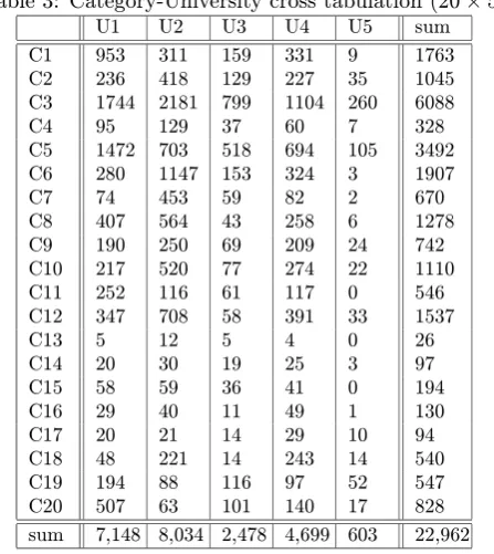
For ourmedia department case, totally 22,962 keywords are selected from their syllabuses. Cross table for 20 cat-egories (clusters) and 5 universities is shown in Table 3. We can perform the considerations on this (20×5) table.
cor-Table 2: 20 term-categories for curriculum analysis
Category
C1 Knowledge and academics, Information science
C2 Psychology
C3 Social Sciences, Economics, Statistics, Sociology, Education C4 Natural Sciences
C5 Mathematics
C6 Physics
C7 Chemistry
C8 Technology and Engineering C9 Construction, Civil engineering C10 Architecture
C11 Mechanical engineering, Nuclear engineering C12 Electrical and Electronic engineering C13 Maritime and Naval engineering C14 Metal and Mining engineering C15 Chemical technology
C16 Manufacturing
C17 Domestic arts and sciences
C18 Commerce, Transportation and Traffic, Communications C19 Music and Dance, Theater, Motion Pictures, Recreation
C20 Language
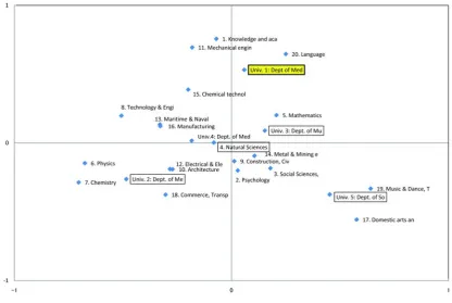
respondence analysis [6]. In this case, term frequencies are standardized to the total value in each university. Eigenvalues for the analysis are {0.0994, 0.0650, 0.0207, 0.0065}. Therefore, it is sufficient to analyze in two di-mensions because the accumulated contribution ratio is 86% for first and second values. Figure 1 shows two-dimension graphical allocation so that we can grasp the global feature of Table 3. Points in thefigure correspond to the vectors of categories (x1
1, x12) and universities (x2
1, x22).
We can obtain global understanding on this curriculum comparison. Interpretations for Figure 1 are as follows: (1) Top center part is an area of computer science or lan-guage. University 1 is related to these categories. (2) Lower right is an area of social science or psychology. University 5 is related to this category. (3) Lower left is an area of natural science and physics. University 2 is related to these categories. (4) University 3 and Univer-sity 4 are located in center area and they have various syllabuses. These departments of University 3 and 4 are regarded as with average curricula.
2.2
Perturbation in Cross Table
As seen in the previous sub-section, various comprehen-sive considerations on the overall accumulated data can be taken by executing the correspondence analysis. How-ever, elements of the cross table, numbers of keywords in syllabuses inevitably contain uncertainty. Therefore, it is necessary to examine sensitivity of the result of corre-spondence analysis for data perturbation in cross table.
[image:2.595.317.541.86.337.2]When a certain perturbation of cross table would make great change for the result of correspondence analysis, the
Table 3: Category-University cross tabulation (20×5)
U1 U2 U3 U4 U5 sum
C1 953 311 159 331 9 1763
C2 236 418 129 227 35 1045
C3 1744 2181 799 1104 260 6088
C4 95 129 37 60 7 328
C5 1472 703 518 694 105 3492
C6 280 1147 153 324 3 1907
C7 74 453 59 82 2 670
C8 407 564 43 258 6 1278
C9 190 250 69 209 24 742
C10 217 520 77 274 22 1110
C11 252 116 61 117 0 546
C12 347 708 58 391 33 1537
C13 5 12 5 4 0 26
C14 20 30 19 25 3 97
C15 58 59 36 41 0 194
C16 29 40 11 49 1 130
C17 20 21 14 29 10 94
C18 48 221 14 243 14 540
C19 194 88 116 97 52 547
C20 507 63 101 140 17 828
sum 7,148 8,034 2,478 4,699 603 22,962
interpretation on the data should be very careful. Some-times we have to correct the interpretation if necessary. On the other hand, the result of correspondence analy-sis might not be influenced by the change of cross table. In such robust case, interpretation of the result of corre-spondence analysis has robust and essentially important features. Therefore, it is important to examine mathe-matically the variations by perturbation of cross table.
For ourmediadepartment case, the calculation result of data perturbation for Table 3 is visualized as shown in Figure 2 [4].
Figure 2 shows the case of perturbation on C6 of uni-versities U1 (Department of Media Technology). U1 is located in the Top upper part of eachfigure. In Figure 2, locations of categories and universities are corresponding to the locations in Figure 1. Arrows in thefigures are the vectors of differential coefficients;
µ
dx11 dapq,
dx12 dapq
,
µ
dx21 dapq,
dx22 dapq
.
The (green) arrow in upper part of thefigure means that if the number of keywords in syllabuses of U1 for Clus-ter 6 increase, then U1 moves toleft direction. U1 goes more closer to the group of natural science asphysics or
chemistry.
Therefore, we are able to understand sensitivities, and expect change for the result of correspondence analysis clearly for variations in text analysis.
Figure 1: Result of correspondence analysis: scoresin two dimension for 5 universities and 20 categories.
Figure 2: Sensitivity for C6 of universities Univ.1 (de-partment of Media Technology).
3
Multiple Correspondence Analysis
3.1
Formulation
of
Multiple
Correspon-dence Analysis
Multiple correspondence analysis is an extension of sim-ple correspondence analysis which is related to various forms of multivariate analysis methods as third method of quantification, dual scaling, andhomogeneity analysis
and others, that are essentially based on singular value decomposition (e.g., [6]). In this section, mathematical
considerations on multiple correspondence analysis are discussed.
[image:3.595.55.284.428.574.2]As an example, Table 4 illustrates a part ofrcategorical data for a certain survey. Each row of this table corre-sponds to a binary coding of factors, also called dummy variables.
Table 4: Example of data table G1 G2 · · · Gr
1 0 0 1 1 0 0 0 0 · · · 1 0 2 1 0 0 0 0 1 0 0 · · · 1 0 3 0 1 0 1 0 0 0 0 · · · 0 1 4 0 1 0 0 0 0 1 0 · · · 1 0 5 0 0 1 0 1 0 0 0 · · · 0 1 6 0 1 0 0 0 0 1 0 · · · 0 1
..
. ... ... ... ...
This table is expressed by an indicator matrixGas
G= (G1, G2,· · ·, Gr). (1)
whereGk is a binary matrix that exactly one element in each row is equal to one.
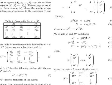
[image:3.595.317.540.525.639.2]vari-ables with categories (As
1, As2,· · ·, Asm) and the variables with categories (At
1, At2,· · ·, Atm). These categories are all inclusive. Each element (ast
ij) shows the number of spe-cific combination of responses to the categories As
i and At
[image:4.595.77.549.68.429.2]j.
Table 5: Cross table forAs×At At1 At2 · · · Atnt As
1 ast11 ast12 · · · ast1nt As
2 ast21 ast22 · · · ast2nt ..
. ... ... ... ... As
ms astms1 amsts2 · · · astmsnt
This cross table for two dimensions is denoted byms×nt matrixAst (sometimes we abbreviatesandt),
Ast= ⎛ ⎜ ⎜ ⎜ ⎝ ast
11 ast12 . . . ast1nt ast
21 ast22 . . . ast2nt ..
. ... ... ... ast
ms1 astms2 . . . astmsnt ⎞ ⎟ ⎟ ⎟
⎠. (2)
The matrix Ast has the following relation with the ma-tricesGsandGt.
Ast= (Gs)TGt (3)
where “T” denotes transform of the matrix.
We denotems×msdiagonal matrix byDs(andnt×nt diagonal matrix by ˜Dt) that has diagonal elements equal to the sum of each column (and row) of the matrix Ast as follows:
Ds= diag(ds11,· · ·, dsmsms), dsii= nt
X
j=1
astij (4)
˜
Dt= diag(dt11,· · ·, dtntnt), dtjj = ms
X
i=1
astij. (5)
It is natural to assume thatdsii >0 anddtjj>0. We have the relation as
Ds = (Gs)TGs (6) ˜
Dt = Gt(Gt)T. (7)
The vectors given to multiple variables are denoted by
xs = (xs
1, . . . , xsms)T , xt = (xt1, . . . , xtnt)T and so on. These vectors are called scoresin correspondence analy-sis. The scores of multiple correspondence analysis are the solutions for the following eigenvalue problem:
⎛ ⎜ ⎜ ⎜ ⎝
D1 A12 . . . A1r A21 D2 . . . A2r ..
. ... ... Ar1 Ar2 . . . Dr
⎞ ⎟ ⎟ ⎟ ⎠ ⎛ ⎜ ⎜ ⎜ ⎝ x1 x2 .. . xr ⎞ ⎟ ⎟ ⎟ ⎠
= r λ
⎛ ⎜ ⎜ ⎜ ⎝
D1 0 D2
. ..
0 Dr
⎞ ⎟ ⎟ ⎟ ⎠ ⎛ ⎜ ⎜ ⎜ ⎝ x1 x2 .. . xr ⎞ ⎟ ⎟ ⎟ ⎠. (8)
Namely,
GTGx = rλDx (9)
D = diag(GTG) (10)
wherex= (x1T,· · ·,xrT)T.
We denoteus andHst as follows:
us = (Ds)12xs (11)
(Ds)12
ii =
p
ds
ii (12)
Hst = (Ds)−12Ast( ˜Dt)− 1
2. (13)
Then, K ⎛ ⎜ ⎜ ⎜ ⎝ u1 u2 .. . ur ⎞ ⎟ ⎟ ⎟ ⎠=rλ
⎛ ⎜ ⎜ ⎜ ⎝ u1 u2 .. . ur ⎞ ⎟ ⎟ ⎟ ⎠ (14)
where the matrixImeans identity matrix,
K= ⎛ ⎜ ⎜ ⎜ ⎝
I1 H12 . . . H1r H21 I2 . . . H2r ..
. ... ...
Hr1 Hr2 . . . Ir ⎞ ⎟ ⎟ ⎟
⎠. (15)
Eigenvalue is denoted byλi, and its corresponding eigen-vector byui which corresponds toxi:
ui= (u1iT,u2iT,· · ·,uriT)T. (16)
Hence
Kui=rλiui. (17)
We haveλi >= 0 in the equation. Moreover, the maximal eigenvalue λ0 = 1 and x0 =1(u0 =D
1
21). Therefore,
we omit this trivial case with λ0 = 1. In the following discussion, we consider the case that the eigenvalues, 0<
λi<1, andλi>=λj for (i < j) and as follows:
0<λi<1, (18)
ui·ui= 1, and ui·uj= 0 (i6=j). (19)
Concerning the value ofχ2we have the following relation:
χ2 = X
s,t,s6=t
σst(tr((Hst)THst)−1)
+X
s ˜
σs(ms−1) (20)
whereσst =P
i,jastij and ˜σs=
P
idsii.
In the case of Section 2, the value ofχ2 is 116.9. Proceedings of the International MultiConference of Engineers and Computer Scientists 2010 Vol I,
3.2
Sensitivity of Multiple Correspondence
Analysis
In this subsection we consider the case that there exists data perturbation in the element of matrixAst. The dif-ferential coefficients of the eigenvectors forast
pq are shown as follows:
(K−λiI)ui=0 (21)
then following equations are obtained according to the characteristics of eigenvalue and eigenvector:
µ
dK dast pq
− dλi dast pq
ui+ (K−λiI) dstu
i dast
pq
=0. (22)
We obtain the following equations with vector standard-ization:
dλi dast pq
= uT i µ dK dast pq 
ui (23)
dui dast pq
= X
j6=i uTj
³ dK dast pq ´ ui
λi−λj
uj (24)
where dK dast pq = ⎛ ⎜ ⎜ ⎜ ⎜ ⎜ ⎝
0 . . . 0 ..
. 0 (dHdastst pq)
.. . ..
. (dHdastst pq)
T 0 ...
0 . . . 0 ⎞ ⎟ ⎟ ⎟ ⎟ ⎟ ⎠ . (25)
We can calculate the value of dHst dast
pq as follows:
dHst dast
pq
=Lstpq+MpstHst+HstNqst (26)
whereLpq, Mp, Nq arem×n, m×m, n×nsparse matri-ces, only one element of that has a value (other elements are zero) as follows:
Lstpq= ⎛ ⎜ ⎝
q
0 ... 0
p · · · √dst1 ppdstqq
0 0
⎞ ⎟
⎠ (27)
Mpst= ⎛ ⎜ ⎝
p
0 ... 0 p · · · − 1
2dst pp 0 0 ⎞ ⎟ ⎠ (28)
Nqst= ⎛ ⎜ ⎝
q
0 ... 0 q · · · −2d1st
0 0
⎞ ⎟
⎠. (29)
We have
dxsi dast pq
=d(D s)−1
2
dast pq
ui+ (Ds)−12 du
s i dast pq
. (30)
Calculating the values of dapqdH , we can easily obtain each numerical value of
µ
dx1 dast pq
, dx2 dast pq
,· · ·
with the matrices
d(Ds)−12
dast pq
.
Using these derivatives, we can visualize the perturba-tions of the scores in correspondence analysis.
Moreover, according similar discussion we can calculate the values of
dχ2 dast pq .
For example, the case of r = 2 that corresponds to the problem in Section tow, we calculate the sensitivity of result of correspondence analysis. The new result is co-incidence to the result of Section two that is shown in Figure 2.
4
Conclusion
In this paper, we consider the sensitivity formultiple cor-respondence analysisand curriculum comparison. Espe-cially, derivatives of the scores for the multiple correspon-dence analysis was deduced. We will refine mathematical discussion on perturbation problem, for example on χ2, and also improve the web-based visualization system for larger sensitivity analysis problem that easily visualizes the results for many variations simultaneously.
References
[1] Nozawa, T., Ida, M., Yoshikane, F., Miyazaki, K. and Kita, H., “Construction of Curriculum Analyz-ing System based on Document ClusterAnalyz-ing of Syl-labus Data”,Journal of Information Processing So-ciety of Japan, Vol. 46, No.1, pp.289—300, 2005.
[2] Ida, M., Nozawa, T., Yoshikane, F., Miyazaki, K. and Kita, H., “Development of Syllabus Database and its Application to Comparative Analysis of Cur-ricula among Majors in Undergraduate Education”,
Research on Academic Degrees and University Eval-uation, Japanese, No.2, pp.85-97, 2005.
6th International Symposium on Advanced Intelli-gent Systems, 2005.
[4] Ida, M, “Textual Information and Correspondence Analysis in Curriculum Analysis”, Proceedings of FUZZIEEE2009, 2009.
[5] NDC, Nippon Decimal Classification, http://en.wikipedia.org/wiki/ Nippon Decimal Classification
[6] Benzecri, J.-P.,Correspondence Analysis Handbook, Marcel Dekker, 1992.