Application of Bhave Toolset for System Control
and Electronic System Design
K.L. Man
∗,
T. Krilaviˇ
cius
†,
C. Chen
‡and H.L. Leung
§Abstract— Behavioural Hybrid Process Calculus (BHPC) is a formalism for modelling and analysis of hybrid systems combining process algebras and the behavioural approach for modelling of instantaneous changes and continuous evolution. BHPC is suppor-ted by Bhave toolset, containing a tool for a novel way of visualisation of hybrid systems simulations msp-svg and a new version of hybrid simulator. We present the latest developments of Bhave toolset and apply it for case studies of system control and mixed-signal systems design.
Keywords: formal methods, electronics, hybrid sys-tems, simulation
1
Introduction
Process algebras/calculi [2,11,19] are formal languages in
Computer Sciencethat have formal syntax and semantics
for specifying and reasoning about different systems. In simple words, process algebras are theoretical frameworks for formal specification and analysis of the behaviour of various systems. Serious efforts have been made in the
past to deal with various systems (e.g.discrete event
sys-tems [20,25],real-time systems [10,12,26] andhybrid
sys-tems [1, 3, 5, 6, 17, 27]) in a process algebraic way. Over
the years, process algebras have been successfully used in a wide range of problems and in practical applications in both academia and industry for analysis of many different systems.
Hybrid systems are systems that exhibit both discrete
and continuous behaviour. Such systems have proved
fruitful in a great diversity of engineering application areas including air-traffic control, automated manufac-turing, chemical process control and system control. On the other hand, mathematically, the behaviour of electro-nic system design (e.g. digital, analog and mixed-signal design) can be described by discrete variables, conti-nuous variables and a set of differential equations, whe-reas switching-modes can be used for modelling mixed
∗Xi’an Jiaotong-Liverpool, University (XJTLU), China, e-mail:
†Vytautas Magnus University (VDU), Kaunas, Lithuania,
e-mail:[email protected].
‡Global Institute of Software Technology, Suzhou, China, e-mail:
§Solari, Hong Kong, e-mail:
models (i.e. mixed-signal design). Due to all these, di-gital, analog and mixed-signal design can be mathemati-cally described as hybrid systems (with various level of abstraction) by nature.
Computer simulationis a powerful tool for analysing and
optimising real-world systems with a wide range of suc-cessful applications. It provides an appealing approach for the analysis of dynamic behaviour of processes and helps decision makers identify different possible options by analysing enormous amounts of data.
Behavioural Hybrid Process Calculus (BHPC) [17] is a hybrid process algebra which was specifically designed for the description of the dynamic behaviour of hybrid
systems along with a powerful simulator called Bhave
toolset. Currently, simulation results obtained by
means of the BHPC simulator can also be visualised and
analysed viaMessage Sequence Plots (MSP) [17].
In this paper, we first present the latest development of
Bhave toolset. Through case studies, we show the
use of Bhave toolsetfor addressing several aspects of
system control and mixed-signal design. Related work of the research activities presented in this paper can be found at [17, 18].
2
Behavioural Hybrid Process Algebra
One of the useful techniques for simulation of hybrid systems that includes continuous evolution and discrete changes, is Behavioural Hybrid Process Calculus (BHPC) [4, 17], an extension of classical process algebra that is suitable for the modelling and analysis of continuous and hybrid dynamical systems and can be seen as a generalisa-tion of the behavioural approach [22] in a hybrid setting. The main strengths of the BHPC are the following.
Sound mathematical foundations. BHPC has sound
mathematical foundations. It means that rigorous reasoning can be applied to investigate diverse pro-perties of models.
Behavioural approach. In BHPC continuous
evolu-tion is defined in the behavioural setting [22] making it more general in contrast to other hybrid process
algebras (Hybridχ[27], HyPA [6], ACPsrths [3]), i.e. it
is defined using trajectories (solutions of differential equations is one of ways of defining trajectories), not just (solutions of) differential equations.
Separation of concerns. Continuous and discrete
be-haviours are specified orthogonally, therefore they can be changed and analysed separately as well as in hybrid setting.
Bisimulation is congruence in BHPC, i.e.
substitu-ting bisimilar (processes, that exhibit the same ob-servable behaviour up-to the branching structure) does not change behaviour of the system.
Tools support. BHPC is supported by Bhave toolset,
see Section 3.
We present main ideas of the BHPC in this section, see [17] for the details.
Trajectories We define trajectories over bounded time
intervals (0, t], and map to a signal space W = (W1×
· · · ×Wn,(q1, . . . , qn)). Components of the signal space
W ∈ W correspond to the different aspects of the
continuous-time behaviour, such as current or voltage,
and are associated withtrajectory qualifiersqi∈ T
iden-tifying them. A trajectory in signal space W is a
func-tion ϕ : (0, t] → W1× · · · ×Wn, where t ∈ R+ is the
duration of the trajectory. We define conditions on the
end-points of trajectories or the exit conditions. ⇓
de-notes such conditions, as the restrictions on the set of
trajectories: Φ ⇓ Predexit={ϕ: (0, u]→W1, . . . , Wn ∈
Φ| Predexit(ϕ(u))}, whereuis a time parameter, Φ is a
set of trajectories and Predexit(ϕ(u)) is a predicate that
defines restrictions. The set of trajectories Φ can be de-fined in different ways, e.g. by ODE/DAE. See [17] for the formal treatment.
Hybrid transition system All behaviours of BHPC
specification are defined by a hybrid transition system
HT S=hS,A,→,W,Φ,→ci
• S is a state space.
• Ais afinite set of (discrete) actions names.
• →⊆S×A×Sis adiscrete transition relations, where
a∈ A. We will denote its−→a s0.
• Wis asignal space.
• Φ is aset of trajectories.
• →c⊆S×Φ×S is a continuous transition relation,
where ϕ∈Φ are trajectories. We will denote
conti-nuous transitionss−→ϕ s0 for the convenience.
Language A core language is used for defining
evolu-tion and interacevolu-tion of systems
B::=0 a. B [f |Φ]. B P
i∈I
Bi BkHA B P
We will require aconsistent signal flow, i.e. only the
pa-rallel composition is allowed to change the set of trajec-tory qualifiers in the process.
Only a subset of complete language is introduced, see [17] for auxiliary operators, such as renaming or hiding. Mo-reover, other operators can be defined on top of the core language for convenience. We demonstrate it by
introdu-cingparametrised action prefix andguard.
Stop 0is the process that does not exhibit any behaviour.
Action prefix a. B performs a and continues as B. A
special silent action τ defines directly unobservable
be-haviour, and is usually used to specify a non-determinism
(e.g. asinternal actionsin [19, p. 37–43]).
We will use parametrisation of action prefix as in [19, p.
53–58]a(v:V). B(v) = P
v∈V
a(v). B(v).
Trajectory prefix[f |Φ]. B(f), wheref is a trajectory
variable, starts with a trajectory or a prefix of a trajectory from the set of trajectories Φ. If a trajectory or a part of it was taken and there exists a continuation of the trajectory, then the system can continue with a trajectory from the set of such continuations. If a whole trajectory (e.g., as defined by exit conditions) was taken, then the system can continue with B.
Choice P{B(v) | v ∈ I} is a generalised
nondetermi-nisticchoice of processes (I is an arbitrary index set). It
chooses before taking an action prefix or trajectory prefix.
Binary version of choice is denoted byB1+B2.
Parallel composition B1 kHA B2, where A and H are
sets of synchronising action names and trajectory qua-lifiers, respectively, models the behaviour of two parallel processes. Synchronisation on actions has an interleaving semantics. Trajectory prefixes evolve only in parallel, and only if the evolution of the coinciding trajectory qualifiers is equal.
Recursions allows defining processes in terms of each
other, as in the equationP =B, whereP is the process
identifier and B is a process expression that may only
contain actions and signal types of B.
GuardhPredioperator evaluatesPred conditions, and if
they are not satisfied, stops the progress of the process.
hPred(x)i. B(x) = P
w|=Pred(w)
B(w)
Herex are process parameters (variables).
Strong bisimulation for hybrid transition systems re-quires both systems to be able to execute the same trajec-tories and actions and to have the same branching struc-ture.
Thehybrid strong bisimulation relation (equivalence)
de-fined for the HTS is a congruence relation w.r.t. all ope-rations defined above [17]. Hence, bisimilar components can be interchanged without changing systems behaviour, and that can be effectively employed while building and improving systems (models).
3
Bhave toolset
BHPC is supported by Bhave toolset [13]. The toolset allows modelling, simulation and visualisation of the hy-brid models [14]. It consists of several tools.
Discrete Bhave [16] allows discrete simulation of the
BHPC specifications.
Bhave simulator allows hybrid simulation of BHPC
specifications. Current version supports a subset of BHPC. A snapshot of the system with examples is
available frombhpc-simulator.sourceforge.net.
BHPC2Mod can translate a restricted set of BHPC
models to Modelica [9] language, and then simulate them using Dymola [8] or OpenModelica [21]. Ho-wever, because Modelica does not have formal se-mantics, translation does not necessary preserves all the properties. Moreover, parallel composition is not translated [28].
msp-svg is a visualisation tool that uses Message
Se-quence Plots (MSP) [17, 24] approach for visualising
hybrid evolution. It is available athttp://msp-svg.
sourceforge.net/. See Section 3.1 for details about
msp-svg.
The current versions of both tools (Bhaveandmsp-svg)
are built not just as a prototypes, but also as a hybrid “sand-box”, a place to experiment with BHPC and re-lated developments. Architecture and implementation of the both tools allows accommodating diverse changes and test the algorithms developed for BHPC or other (hybrid) process algebras or MSP-based visualisation techniques comparatively easy.
Our plans include further development of the process
al-gebra andBhave toolset. We are planning to improve
and extendBhaveand integrate it withmsp-svg.
3.1
Visualisation of Hybrid Evolutions
Simulation results usually visualise the evolution of the system in time. Event traces or message sequence charts
(MSC) [23] adequately represent discrete system beha-viour, and graphs are convenient for the ordinary conti-nuous systems. However, in hybrid systems we have both the evolution of system variables and events. Hence, a combined view is crucial to fully analyse hybrid system behaviour. See [17, p. 118-124] for the details.
We believe, that Message Sequence Plots (MSP) [17, p. 118-124] contains all necessary components for ade-quate visualisation of hybrid systems. It has two
com-pounds: message-sequence charts rotated 90◦ combined
with plots. We explain MSP by an example depicted in Figure 1.
Plots over time-lines show continuous-time evolution.
A legend allows selecting qualifiers of interest, that
are depicted in the plot. If several processes
evolve concurrently, the synchronising qualifiers
ap-pear for both processes. In Figure 1 qualifiers
qual1,qual2,qual3and qual4are depicted. Processi
is related with qualifiersqual1,qual2 andqual3, and
only qualifiersqual1andqual3 are selected to be
vi-sible. Processjis related with qualifiersqual1,qual2
andqual4, and qualifiersqual2andqual4are selected
to be visible.
Single horizontal lines connected to the
correspon-ding boxes with process identifiers, represent
pro-cesses and the time-line (or life-line in MSC
ter-minology). Time is assumed to flow to the right
along each time-line at the same speed. Processi
andProcessjare represented by the horizontal lines
and boxes with processes identifiers in the example.
Labelled vertical lines going across time-lines
re-present communication, i.e. (parameterised) action prefixes in BHPC. Notice that we use simple lines instead of arrows, because communication in BHPC
is not directed. Communication of Processi and
Processjconsists of actionsact1,act2 andact3.
Triple horizontal time-lines depict suspension of the
time-flow. Single actions are placed on the time-line at the time that relates to their moment of occur-rence. A sequence of actions occurs at one moment in time, when there is no continuous behaviour bet-ween the actions. We suspend the flow of time to allow insight in the ordering of these actions. In the example, suspension of the time is depicted on the time-line as three parallel solid lines.
Figure 1 contains all information that would be available
in an ordinary plot. Correspondingly, all information
that is visible in message sequence charts, is also visible in MSP. Furthermore, in MSP all processes and com-munication between them are visualised. The proposed technique can be easily adopted to other hybrid system
□ □ □vv
qual1 qual2 qual3 □ □ □ v v qual1 qual2 qual4
act1act2act3 act3
Processi
[image:4.612.300.548.70.224.2]Processj
Figure 1: MSP example.
988.000 957.000 926.000 895.000 864.000 833.000 802.000 771.000 741.000 710.000 679.000 648.000 617.000 586.000 556.000 526.000 495.000 464.000 434.000 403.000 simpleVessel 0.707 -2.000 1.127 -1.870 1.546 -1.739 1.966 -1.609 2.385 -1.478 2.804 -1.348 3.224 -1.217 3.643 -1.087 4.063 -0.957 4.482 -0.826 4.902 -0.696 5.321 -0.565 5.741 -0.435 6.160 -0.304 6.580 -0.174 6.999 -0.043 7.419 0.087 7.838 0.217 8.258 0.348 8.677 0.478 9.097 0.609 9.516 0.739 9.936 0.870 40.167 42.524 44.882 47.240 49.598 51.956 54.314 56.671 59.029 61.387 63.745 66.103 68.461 70.819 73.176 75.534 77.892 80.250 82.608 84.966 87.324 89.681 92.039 94.397 fi llOff. on fi llOn. o ff fi llOff. on fi llOn. o ff fi llOff. o n fi llOn. off fi llOff. o n
time, ( 40.167; 96.755)
simpleVessel.level, ( 0.707; 10.355)
simpleVessel.level' ( -2.000; 1.000)
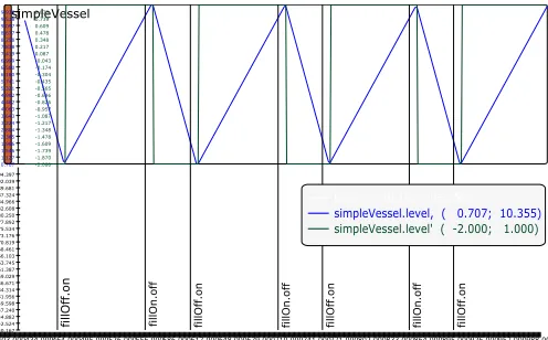
Figure 2: Simulation of the simple vessel.
modelling frameworks with minimal changes, e.g., if com-munication is directed, arrows can be used to depict it.
Additional notation, such as decorating the results with process expressions (e.g. action and trajectory prefixes), adding recursive calls, providing information about rena-ming of qualifiers in the legend, forking of processes to depict parallelism. See [15] for details.
Figure 2 depicts an evolution of the simple vessel
simula-tion 4.1 using a proof of concept tool msp-svg.
Exe-cutable and source code of msp-svg are available at
sourceforge.net/projects/msp-svg/.
4
Application of BHPC
4.1
Simple Vessel
Simple vessel models a system with a constant outflow
of fluid (lout) and controlled inflow (lin ≥ lout). Level
of the fluid should be maintained in a certain interval
[lmin, lmax]. Inflow is controlled by opening (open) and
closing (close) a valve.
We provide a model in BHPC that simulates behaviour of such systems.
SimpleVessel(level) =
OutFlow(level)[simpleVessel.level/level];
InFlow(level) =
[ level’ = (3 - 2) |
(level - 10 - 0.5 * rand()) ] . off
. OutFlow(level)[InFlow.level/level];
OutFlow(level) =
[ level’ = (0 - 2) |
(level - 1 + 0.5 * rand()) ] . on
. InFlow(level)[OutFlow.level/level];
It consists of main process SimpleVessel and two
sub-processes SimpleVessel, InFlow and OutFlow, that,
respectively, simulate inflow and outflow modes.
Swit-ching occurs in the predefined ranges, i.e. the
sys-tem switches to inflow mode when level ∈ [lmin, lon] (in
our case level ∈ [0.5,1.5] ) and to outflow mode when
level ∈ [loff, lmax] ([9.5,10.5]). Ranges allow to model
measuring devices errors and delays. We model non
de-terminism usingrand()function, but in the future we are
planning to introduce other techniques [17, p.115-117] for
it. Inflow and outflow are, respectively 3 and −2 units
of fluid per time unit. Simulation results are depicted in Figure 2. Slanted (blue) lines depict growing and decrea-sing level. Inflow and outflow speed (derivatives of fluid level change) are depicted by black horizontal lines,
res-pectively, at level 1 and−2 (notice, different axes) in the
upper part of the figure. Actions are depicted by vertical lines, and shown in the lower part of the figure.
4.2
Application of BHPC for Tunnel Diode
Modelling
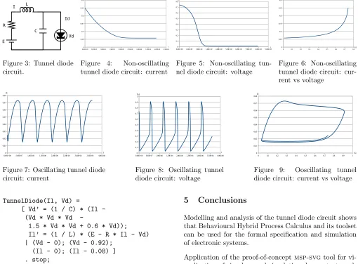
We present results of experiments with the tunnel-diode circuit from [7]. The circuit is depicted in Figure 3. State of the system is defined by two state variables: the
cur-rent through the inductor Il and the voltage across the
diodeVd. Behaviour is defined by differential equations
˙
Il=
1
C(−Id(Vd) +Il) (1)
˙
Vd=
1
L(E−RIl−Vd). (2)
where
Id(Vd) =Vd3−1.5V
2
d + 0.6Vd
defines non-linear characteristics of the tunnel diode.
We provide a simple model of the system, that consists of
one process, namelyTunnelDiode, that contains a
tra-jectory prefix defining evolution of the circuit over time. Exit conditions of the trajectory prefix define expected
intervals for the currentIl and voltageVd.
[image:4.612.49.271.92.229.2]R L I
E
C
Vd Id
Figure 3: Tunnel diode circuit.
0,00E+000 5,00E-09 1,00E-08 1,50E-08 2,00E-08 2,50E-08 3,00E-08 3,50E-08 4,00E-08 4,50E-08 0,005
0,01 0,015 0,02 0,025 0,03
t Il
Figure 4: Non-oscillating
tunnel diode circuit: current
0,00E+00 1,00E+02 2,00E+02 3,00E+02 4,00E+02 5,00E+02 6,00E+02 7,00E+02 8,00E+02 9,00E+02 0
0,1 0,2 0,3 0,4 0,5 0,6 0,7 0,8
t Vd
Figure 5: Non-oscillating tun-nel diode circuit: voltage
0 0,1 0,2 0,3 0,4 0,5 0,6 0,7 0,8
0 0,005 0,01 0,015 0,02 0,025 0,03
Vd Il
Figure 6: Non-oscillating tunnel diode circuit: cur-rent vs voltage
0,00E+00 5,00E-07 1,00E-06 1,50E-06 2,00E-06 2,50E-06 3,00E-06 3,50E-06 4,00E-06 0
0,01 0,02 0,03 0,04 0,05 0,06 0,07 0,08
[image:5.612.43.553.76.452.2]t Il
Figure 7: Oscillating tunnel diode circuit: current
0,00E+000 5,00E-07 1,00E-06 1,50E-06 2,00E-06 2,50E-06 3,00E-06 3,50E-06 4,00E-06 0,1
0,2 0,3 0,4 0,5 0,6 0,7 0,8 0,9 1
t Vd
Figure 8: Oscillating tunnel diode circuit: voltage
0 0,1 0,2 0,3 0,4 0,5 0,6 0,7 0,8 0,9 1 0
0,01 0,02 0,03 0,04 0,05 0,06 0,07 0,08
Vc Il
Figure 9: Ooscillating tunnel
diode circuit: current vs voltage
TunnelDiode(Il, Vd) =
[ Vd’ = (1 / C) * (Il -(Vd * Vd * Vd
-1.5 * Vd * Vd + 0.6 * Vd)); Il’ = (1 / L) * (E - R * Il - Vd) | (Vd - 0); (Vd - 0.92);
(Il - 0); (Il - 0.08) ] . stop;
We performed simulation with two different sets of para-meters.
Non-oscillating Oscillating
C(F) 10−9 10−9
L(H) 10−6 10−6
E(V) 0.3 10−9
R(Ω) 50 0.3
Initial values: Il= 0.025Aand Vd= 0.74V. Notice, that
only voltage differs.
As expected, in the first case simulation stabilises in the equilibrium. Figures 4, 5 and 6 depict the current, voltage and current vs voltage of the non-oscillating tunnel diode circuit, respectively.
With the second set of parameters we get an oscillating system in the expected intervals. Simulation of the oscil-lating tunnel diode circuit is depicted in Figures 7, 8 and 9.
5
Conclusions
Modelling and analysis of the tunnel diode circuit shows that Behavioural Hybrid Process Calculus and its toolset can be used for the formal specification and simulation of electronic systems.
Application of the proof-of-concept msp-svgtool for
vi-sualisation of simple vessel simulation demonstrates ad-vantages of the Message Sequence Plots over simple plots, because not only switching points are visible, but a cause (a related event) as well.
Our future work will focus on several aspects.
• Application of the toolset to analog and mixed
elec-tronic systems.
• Modular specifications of diverse circuits, i.e.
model-ling of circuits as parallel components, e.g. modelmodel-ling tunnel diode circuit as parallel interconnection of ca-pacitor, inductor, resistor, tunnel diode and power source.
• Improvements of the modelling language. Currently
we use the language, that consists only of basic constructs. We are planning to add some syntactical constructs for convenience.
• Improvements of tools. We are planning to improve
simulator andmsp-svgtools, integrate them.
References
[1] R. Alur, C. Courcoubetis, N. Halbwachs, T. A. Hen-zinger, P. H. Ho, X. Nicollin, A. Olivero, J. Sifakis, and S. Yovine. The algorithmic analysis of hybrid
systems. TCS, 138(1):3–34, 1995.
[2] J. C. M. Baeten and W. P. Weijland. Process
Al-gebra, volume 18 of Camb. Tracts in TCS. Camb.
Univ. Press, Cambridge, UK, 1990.
[3] J. A. Bergstra and C. A. Middelburg. Process
Al-gebra for Hybrid Systems. TCS, 335(2/3):215–280,
2005.
[4] E. Brinksma, T. Krilaviˇcius, and Y. S. Usenko.
Pro-cess Algebraic Approach to Hybrid Systems. InProc.
of 16th IFAC World Congress, pages 1–6, Prague,
Czech Rep., July 2005.
[5] L. P. Carloni, R. Passerone, A. Pinto, and A. L.
Sangiovanni-Vincentelli. Language and Tools for
Hybrid Systems Design. J of Found. and Trends,
1:1–177, 2005.
[6] P. J. L. Cuijpers and M. A. Reniers. Hybrid Process
Algebra. JLAP, 62(2):191–245, 2005.
[7] W. Denman. Formal Verification of Analog and
Mixed Signal Designs. Master’s thesis, Concordia Univ., 2009.
[8] Dynasim, 2006. Last accessed: 2006 May 11.
[9] P. Fritzson and V. Engelson. Modelica - A
Uni-fied Object-Oriented Language for System Modelling and Simulation, 1998.
[10] M. Geilen. Formal Techniques for Verification of
Complex Real-time Systems. PhD thesis, Tech. Univ.
of Eindhoven, 2001.
[11] C. A. R. Hoare. Communicating Sequential
Pro-cesses. Prent.-Hall, 1985.
[12] J. Hooman. Specification and Compositional
Verifi-cation of Real-Time Systems. Springer, 1991.
[13] T. Krilaviˇcius. Bhave :: Simulation of Hybrid
Sys-tems, 2006.
[14] T. Krilaviˇcius. Simulation of Mechatronic Systems
Using Behavioural Hybrid Process Calculus.
Elec-tron. and Elec. Eng., 1(81):45–48, 2008.
[15] T. Krilaviˇcius and K.L. Man.Intelligent Automation
and Computer Engineering, chapter Behavioural
Hy-brid Process Calculus for Modelling and Analysis of Hybrid and Electronic Systems. Springer, 2009.
[16] T. Krilaviˇcius and H. Schonenberg. Discrete
Simu-lation of Behavioural Hybrid Process Calculus. In
P. M. E. Bra and J. J. van Wijk, editors, IFM2005
Doctoral Symposium, pages 33–38, Eindhoven,
Ne-therlands, November 2005. Tech. Univ. of Eindho-ven, Dept. of Math. and CS.
[17] T. Krilavˇcius. Hybrid Techniques for Hybrid
Sys-tems. PhD thesis, Univ. of Twente, 2006.
[18] K. L. Man and M. P. Schellekens. Current Trends
in Intelligent Systems and Computer Engineering,
chapter Interoperability of Performance and Func-tional Analysis for Electronic System Designs in Be-havioural Hybrid Process Calculus (BHPC). Sprin-ger, 2008.
[19] R. Milner.Communication and Concurrency.
Pren.-Hall, 1989.
[20] G. Naumoski and W. Alberts. A Discrete-Event
Si-mulator for Systems Engineering. PhD thesis, Tech.
Univ. of Eindhoven, 1998.
[21] OpenModelica System website. OpenModelica
System, 2009. http://www.ida.liu.se/~pelab/
modelica/OpenModelica.html.
[22] J. W. Polderman and J. C. Willems. Introduction
to Mathematical Systems Theory: a behavioral
ap-proach. Springer, 1998.
[23] E. Rudolph, P. Graubmann, and J. Grabowski.
Tu-torial on Message Sequence Charts. Comput. Netw.
ISDN Syst., 28(12):1629–1641, 1996.
[24] M. H. Schonenberg. Discrete Simulation of
Beha-vioural Hybrid Process Algebra. Master’s thesis,
Univ. of Twente, 2006. Master thesis.
[25] D. A. van Beek, S. H. F. Gordijn, and J. E. Rooda. Integrating Continuous-Time and Discrete-Event Concepts in Modelling and Simulation of
Ma-nufacturing Machines. Sim. Pract. and Theory,
5(7-8):653–669, 1997.
[26] D. A. van Beek, K. L. Man, M. A. Reniers, J. E.
Rooda, and R. R. H. Schiffelers. Syntax and
se-mantics of timed Chi. Technical Report CS-Report 05-09, Tech. Univ. of Eindhoven, Dept. of CS, The Netherlands, 2005.
[27] D. A. van Beek, K. L. Man, M. A. Reniers,
J. E. Rooda, and R. R. H. Schiffelers. Syntax
and Consistent Equation Semantics of Hybrid Chi.
JLAP, 68(1-2):129–210, 2006.
[28] A. van Putten. Behavioural Hybrid Process Calculus Parser and Translator to Modelica. Master’s thesis, Univ. of Twente, 2006.