Investigating the Effects of Selective Sampling on the Annotation Task

Investigating the Effects of Selective Sampling on the Annotation Task

Ben Hachey, Beatrice Alex and Markus Becker School of Informatics

University of Edinburgh Edinburgh, EH8 9LW, UK

{bhachey,v1balex,s0235256}@inf.ed.ac.uk

Abstract

We report on an active learning experi-ment for named entity recognition in the astronomy domain. Active learning has been shown to reduce the amount of la-belled data required to train a supervised learner by selectively sampling more in-formative data points for human annota-tion. We inspect double annotation data from the same domain and quantify poten-tial problems concerning annotators’ per-formance. For data selectively sampled according to different selection metrics, we find lower inter-annotator agreement and higher per token annotation times. However, overall results confirm the util-ity of active learning.

1 Introduction

Supervised training of named entity recognition (NER) systems requires large amounts of manually annotated data. However, human annotation is typ-ically costly and time-consuming. Active learn-ing promises to reduce this cost by requestlearn-ing only those data points for human annotation which are highly informative. Example informativity can be estimated by the degree of uncertainty of a single learner as to the correct label of a data point (Cohn et al., 1995) or in terms of the disagreement of a committee of learners (Seung et al., 1992). Ac-tive learning has been successfully applied to a va-riety of tasks such as document classification (Mc-Callum and Nigam, 1998), part-of-speech tagging

(Argamon-Engelson and Dagan, 1999), and parsing (Thompson et al., 1999).

We employ a committee-based method where the degree of deviation of different classifiers with re-spect to their analysis can tell us if an example is potentially useful. In a companion paper (Becker et al., 2005), we present active learning experiments for NER in radio-astronomical texts following this approach.1 These experiments prove the utility of selective sampling and suggest that parameters for a new domain can be optimised in another domain for which annotated data is already available.

However there are some provisos for active learn-ing. An important point to consider is what effect

informative examples have on the annotators. Are

these examples more difficult? Will they affect the annotators’ performance in terms of accuracy? Will they affect the annotators performance in terms of time? In this paper, we explore these questions us-ing doubly annotated data. We find that selective sampling does have an adverse effect on annotator accuracy and efficiency.

In section 2, we present standard active learn-ing results showlearn-ing that good performance can be achieved using fewer examples than random sam-pling. Then, in section 3, we address the questions above, looking at the relationship between inter-annotator agreement and annotation time and the ex-amples that are selected by active learning. Finally, section 4 presents conclusions and future work.

1

Please refer to the companion paper for details of the selective sampling approach with experimental adaptation re-sults as well as more information about the corpus of radio-astronomical abstracts.

2 BootstrappingNER

The work reported here was carried out in order to assess methods of porting a statisticalNERsystem to

a new domain. We started with aNERsystem trained on biomedical literature and built a new system to identify four novel entities in abstracts from astron-omy articles. This section introduces the Astronastron-omy Bootstrapping Corpus (ABC) which was developed for the task, describes our active learning approach to bootstrapping, and gives a brief overview of the experiments.

2.1 The Astronomy Bootstrapping Corpus

The ABC corpus consists of abstracts of radio astro-nomical papers from the NASA Astrophysics Data System archive2, a digital library for physics, as-trophysics, and instrumentation. Abstracts were ex-tracted from the years 1997-2003 that matched the query “quasar AND line”. A set of 50 abstracts from the year 2002 were annotated as seed mate-rial and 159 abstracts from 2003 were annotated as testing material. A further 778 abstracts from the years 1997-2001 were provided as an unannotated pool for bootstrapping. On average, these abstracts contain 10 sentences with a length of 30 tokens. The annotation marks up four entity types:

Instrument-name (IN) Names of telescopes and other measurement instruments, e.g.

Superconduct-ing Tunnel Junction (STJ) camera, Plateau de Bure Interferometer, Chandra, XMM-Newton Reflection Grating Spectrometer (RGS), Hubble Space Tele-scope.

Source-name (SN) Names of celestial objects, e.g. NGC 7603, 3C 273, BRI 1335-0417, SDSSp

J104433.04-012502.2, PC0953+ 4749.

Source-type (ST) Types of objects, e.g. Type II

Su-pernovae (SNe II), radio-loud quasar, type 2 QSO, starburst galaxies, low-luminosity AGNs.

Spectral-feature (SF) Features that can be pointed to on a spectrum, e.g. Mg II emission, broad

emission lines, radio continuum emission at 1.47 GHz, CO ladder from (2-1) up to (7-6), non-LTE line.

2_{http://adsabs.harvard.edu/preprint_}

service.html

The seed and test data sets were annotated by two astrophysics PhD students. In addition, they anno-tated 1000 randomly sampled sentences from the pool to provide a random baseline for active learn-ing. These sentences were doubly annotated and ad-judicated and form the basis for our calculations in section 3.

2.2 Inter-Annotator Agreement

In order to ensure consistency in annotation projects, corpora are often annotated by more than one an-notator, e.g. in the annotation of the Penn Treebank (Marcus et al., 1994). In these cases, inter-annotator agreement is frequently reported between different annotated versions of a corpus as an indicator for the difficulty of the annotation task. For example, Brants (2000) reports inter-annotator agreement in terms of accuracy and f-score for the annotation of the German NEGRA treebank.

Evaluation metrics for named entity recognition are standardly reported as accuracy on the token level, and as f-score on the phrasal level, e.g. Sang (2002), where token level annotation refers to the B-I-O coding scheme.3 Likewise, we will use accuracy to report inter-annotator agreement on the token level, and f-score for the phrase level. We may arbitrarily assign one annotator’s data as the gold standard, since both accuracy and f-score are symmetric with respect to the test and gold set. To see why this is the case, note that accuracy can sim-ply be defined as the ratio of the number of tokens on which the annotators agree over the total number of tokens. Also the f-score is symmetric, since re-call(A,B) = precision(B,A) and (balanced) f-score is the harmonic mean of recall and precision (Brants, 2000). The pairwise f-score for the ABC corpus is 85.52 (accuracy of 97.15) with class information and 86.15 (accuracy of 97.28) without class information. The results in later sections will be reported using this pairwise f-score for measuring agreement.

For NER, it is also common to compare an anno-tator’s tagged document to the final, reconciled ver-sion of the document, e.g. Robinson et al. (1999) and Strassel et al. (2003). The inter-annotator f-score agreement calculated this way for MUC-7 and Hub 4 was measured at 97 and 98 respectively. The

3

doubly annotated data for the ABC corpus was re-solved by the original annotators in the presence of an astronomy adjudicator (senior academic staff) and a computational linguist. This approach gives an f-score of 91.89 (accuracy of 98.43) with class information for the ABC corpus. Without class in-formation, we get an f-score of 92.22 (accuracy of 98.49), indicating that most of our errors are due to boundary problems. These numbers suggest that our task is more difficult than the genericNERtasks from the MUC and HUB evaluations.

Another common agreement metric is the kappa coefficient which normalises token level accuracy by chance, e.g. Carletta et al. (1997). This met-ric showed that the human annotators distinguish the four categories with a reproducibility of K=.925 (N=44775, k=2; where K is the kappa coefficient, N is the number of tokens and k is the number of annotators).

2.3 Active Learning

We have already mentioned that there are two main approaches in the literature to assessing the informa-tivity of an example: the degree of uncertainty of a single learner and the disagreement between a com-mittee of learners. For the current work, we employ query-by-committee (QBC). We use a conditional Markov model (CMM) tagger (Klein et al., 2003; Finkel et al., 2005) to train two different models on the same data by splitting the feature set. In this sec-tion we discuss several parameters of this approach for the current task.

Level of annotation For the manual annotation of named entity examples, we needed to decide on the level of granularity. The question arises of what con-stitutes an example that will be submitted to the an-notators. Possible levels include the document level, the sentence level and the token level. The most fine-grained annotation would certainly be on the token level. However, it seems unnatural for the annota-tor to label individual tokens. Furthermore, our ma-chine learning tool models sequences at the sentence level and does not allow to mix unannotated tokens with annotated ones. At the other extreme, one may submit an entire document for annotation. A possi-ble disadvantage is that a document with some inter-esting parts may well contain large portions with

re-dundant, already known structures for which know-ing the manual annotation may not be very useful. In the given setting, we decided that the best granu-larity is the sentence.

Sample Selection Metric There are a variety of metrics that could be used to quantify the degree of deviation between classifiers in a committee (e.g. KL-divergence, information radius, f-measure). The work reported here uses two sentence-level met-rics based on KL-divergence and one based on f-measure.

KL-divergence has been used for active learning

to quantify the disagreement of classifiers over the probability distribution of output labels (McCallum and Nigam, 1998; Jones et al., 2003). It measures the divergence between two probability distributions pandqover the same event spaceχ:

D(p||q) =X

x∈χ

p(x) logp(x)

q(x) (1)

KL-divergence is a non-negative metric. It is zero for identical distributions; the more different the two distributions, the higher the KL-divergence. Intu-itively, a high KL-divergence score indicates an in-formative data point. However, in the current formu-lation, KL-divergence only relates to individual to-kens. In order to turn this into a sentence score, we need to combine the individual KL-divergences for the tokens within a sentence into one single score. We employed mean and max.

The f-complement has been suggested for active learning in the context of NP chunking as a struc-tural comparison between the different analyses of a committee (Ngai and Yarowsky, 2000). It is the pairwise f-measure comparison between the multi-ple analyses for a given sentence:

f_compM = 1 2

X

M,M0_∈M

(1−F1(M(t), M0(t))) (2)

where F1 is the balanced f-measure of M(t) and

69 70 71 72 73 74 75 76 77 78 79 80

10000 15000 20000 25000 30000 35000 40000 45000

F-score

Number of Tokens in Training Data Ave KL-divergence Random sampling

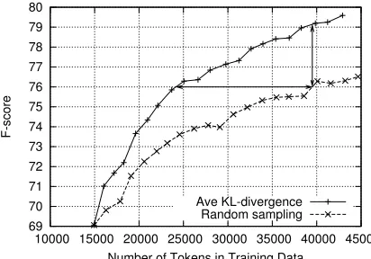
Figure 1: Learning curve of the real AL experiment.

2.4 Experiments

To tune the active learning parameters discussed in section 2.3, we ran detailed simulated experi-ments on the named entity data from the BioNLP shared task of the COLING 2004 International Joint Workshop on Natural Language Processing in Biomedicine and its Applications (Kim et al., 2004). These results are treated in detail in the companion paper (Becker et al., 2005).

We used the CMM tagger to train two different models by splitting the feature set to give multiple views of the same data. The feature set was hand-crafted such that it comprises different views while empirically ensuring that performance is sufficiently similar. On the basis of the findings of the simulation experiments we set up the real active learning anno-tation experiment using: average KL-divergence as the selection metric and a feature split that divides the full feature set roughly into features of words and features derived from external resources. As smaller batch sizes require more retraining iterations and larger batch sizes increase the amount of anno-tation necessary at each round and could lead to un-necessary strain for the annotators, we settled on a batch size of 50 sentences for the real AL experi-ment as a compromise between computational cost and work load for the annotator.

We developed an active annotation tool and ran real annotation experiments on the astronomy ab-stracts described in section 2.1. The tool was given to the same astronomy PhD students for annotation who were responsible for the seed and test data. The learning curve for selective sampling is plotted in

figure 1.4 The randomly sampled data was dou-bly annotated and the learning curve is averaged be-tween the two annotators.

Comparing the selective sampling performance to the baseline, we confirm that active learning pro-vides a significant reduction in the number of exam-ples that need annotating. In fact, the random curve reaches an f-score of 76 after approximately 39000 tokens have been annotated while the selective sam-pling curve reaches this level of performance after only≈24000 tokens. This represents a substantial reduction in tokens annotated of 38.5%. In addition, at 39000 tokens, selectively sampling offers an error reduction of 21.4% with a 3 point improvement in f-score.

3 Evaluating Selective Sampling

Standardly, the evaluation of active learning meth-ods and the comparison of sample selection metrics draws on experiments over gold-standard annotated corpora, where a set of annotated data is at our dis-posal, e.g. McCallum and Nigam (1998), Osborne and Baldridge (2004). This assumes implicitly that annotators will always produce gold-standard qual-ity annotations, which is typically not the case, as we discussed in Section 2.2. What is more, we speculate that annotators might have an even higher error rate on the supposedly more informative, but possibly also more difficult examples. However, this would not be reflected in the carefully annotated and veri-fied examples of a gold standard corpus. In the fol-lowing analysis, we leverage information from dou-bly annotated data to explore the effects on annota-tion of selectively sampled examples.

To evaluate the practicality and usefulness of ac-tive learning as a generally applicable methodology, it is desirable to be able to observe the behaviour of the annotators. In this section, we will report on the evaluation of various subsets of the doubly an-notated portion of the ABC corpus comprising 1000 sentences, which we sample according to a sample selection metric. That is, examples are added to the subsets according to the sample selection metric, se-lecting those with higher disagreement first. This allows us to trace changes in inter-annotator

agree-4

ment between the full corpus and selected subsets thereof. Also, we will inspect timing information. This novel methodology allows us to experiment with different sample selection metrics without hav-ing to repeat the actual time and resource intensive annotation.

3.1 Error Analysis

To investigate the types of classification errors, it is common to set up a confusion matrix. One approach is to do this at the token level. However, we are deal-ing with phrases and our analysis should reflect that. Thus we devised a method for constructing a confu-sion matrix based on phrasal alignment. These con-fusion matrices are constructed by giving a double count for each phrase that has matching boundaries and a single count for each phrase that does not have matching boundaries. To illustrate, consider the fol-lowing sentences–annotated with phrasesA, B, and Cfor annotator 1 on top and annotator 2 on bottom– as sentence 1 and sentence 2 respectively:

A A

B

A C

A

B

A C

A

Sentence 1 will get a count of 2 for A/A and for A/B and a count of 1 for O/C, while sentence 2 will get 2 counts ofA/O, and 1 count each of O/A, O/B, and O/C. Table 1 contains confusion matrices

for the first 100 sentences sorted by averaged KL-divergence and for the full set of 1000 random sen-tences from the pool data. (Note that these confusion matrices contain percentages instead of raw counts so they can be directly compared.)

We can make some interesting observations look-ing at these phrasal confusion matrices. The main effect we observed is the same as was suggested by the f-score inter-annotator agreement errors in sec-tion 2.1. Specifically, looking at the full random set of 1000 sentences, almost all errors (Where∗is any entity phrase type, ∗/O_{all errors}+O/∗errors = 95.43%) are due to problems with phrase boundaries. Compar-ing the full random set to the 100 sentences with the highest averaged KL-divergence, we can see that this is even more the case for the sub-set of 100 sen-tences (97.43%). Therefore, we can observe that

100: A2

IN SN ST SF O

IN 12.0 0.0 0.0 0.0 0.4

SN 0.0 10.4 0.0 0.0 0.4

A1 ST 0.0 0.4 30.3 0.0 1.0

SF 0.0 0.0 0.0 31.1 3.9

O 0.2 0.4 2.9 6.4 —

1000: A2

IN SN ST SF O

IN 9.4 0.0 0.0 0.0 0.3

SN 0.0 10.1 0.2 0.1 0.3 A1 ST 0.0 0.1 41.9 0.1 1.6 SF 0.0 0.0 0.1 25.1 3.0 O 0.3 0.2 2.4 4.8 —

Table 1: Phrasal confusion matrices for document sub-set of 100 sentences sorted by average KL-divergence and for full random document sub-set of 1000 sentences (A1: Annotator 1, A2: Annotator 2).

Entity 100 1000

Instrument-name 12.4% 9.7%

Source-name 10.8% 10.7%

Source-type 31.7% 43.7%

Spectral-feature 35.0% 28.2%

O 9.9% 7.7%

Table 2: Normalised distributions of agreed entity annotations.

there is a tendency for the averaged KL-divergence selection metric to choose sentences where phrase boundary identification is difficult.

Furthermore, comparing the confusion matrices for 100 sentences and for the full set of 1000 shows that sentences containing less common entity types tend to be selected first while sentences containing the most common entity types are dispreferred. Ta-ble 2 contains the marginal distribution for annotator 1 (A1) from the confusion matrices for the ordered sub-set of 100 and for the full random set of 1000 sentences. So, for example, the sorted sub-set con-tains 12.4%Instrument-nameannotations (the least common entity type) while the full set con-tains 9.7%. And, 31.7% of agreed entity annota-tions in the first sub-set of 100 areSource-type

0.87 0.88 0.89 0.9 0.91 0.92 0.93 0.94 0.95 0.96 0.97 0.98

0 5000 10000 15000 20000 25000 30000

Inter-annotator Agreement (Acc)

Size (Tokens) of KL-sorted Document Subset KL-divergence

Figure 2: Raw agreement plotted against KL-sorted document subsets.

tion of agreed Source-type annotations in the full random set is 43.7%. Looking at the O row, we also observe that sentences with difficult phrases are preferred. A similar effect can be observed in the marginals for annotator 2.

3.2 Annotator Performance

So far, the behaviour we have observed is what you would expect from selective sampling; there is a marked improvement in terms of cost and error rate reduction over random sampling. However, selec-tive sampling raises questions of cogniselec-tive load and the quality of annotation. In the following section we investigate the relationship between informativ-ity, inter-annotator agreement, and annotation time.

While reusability of selective samples for other learning algorithms has been explored (Baldridge and Osborne, 2004), no effort has been made to quantify the effect of selective sampling on anno-tator performance. We concentrate first on the ques-tion: Are informative examples more difficult to

an-notate? One way to quantify this effect is to look

at the correlation between human agreement and the token-level KL-divergence. The Pearson correlation coefficient indicates the degree to which two vari-ables are related. It ranges between−1and1, where 1means perfectly positive correlation, and−1 per-fectly negative correlation. A value of0indicates no correlation. The Pearson correlation coefficient on all tokens gives a very weak correlation coefficient of−0.009.5 However, this includes many trivial

to-5

In order to make this calculation, we give token-level

0.76 0.77 0.78 0.79 0.8 0.81 0.82 0.83 0.84 0.85 0.86

100 200 300 400 500 600 700 800 900 1000

Inter-annotator Agreement (F)

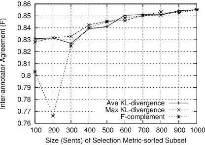
Size (Sents) of Selection Metric-sorted Subset Ave KL-divergence Max KL-divergence F-complement

Figure 3: Human disagreement plotted against se-lection metric-sorted document subsets.

kens which are easily identified as being outside an entity phrase. If we look just at tokens that at least one of the annotators posits as being part of an en-tity phrase, we observe a larger effect with a Pear-son correlation coefficient of−0.120, indicating that agreement tends to be low when KL-divergence is high. Figure 2 illustrates this effect even more dra-matically. Here we plot accuracy against token sub-sets of size1000,2000, .., Nwhere tokens are added to the subsets according to their KL-divergence, se-lecting those with the highest values first. This demonstrates clearly that tokens with higher KL-divergence have lower inter-annotator agreement.

However, as discussed in sections 2.3 and 2.4, we decided on sentences as the preferred annota-tion level. Therefore, it is important to explore these relationships at the sentence level as well. Again, we start by looking at the Pearson correlation coeffi-cient between f-score inter-annotator agreement (as described in section 2.1) and our active learning se-lection metrics:

Ave KL Max KL 1-F All Tokens −0.090 −0.145 −0.143 O Removed −0.042 −0.092 −0.101

Here O Removed means that sentences are removed for which the annotators agree that there are no en-tity phrases (i.e. all tokens are labelled as being outside an entity phrase). This shows a

0.65 0.7 0.75 0.8 0.85 0.9 0.95

100 200 300 400 500 600 700 800 900 1000

Average time per token

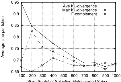
Size (Sents) of Selection Metric-sorted Subset Ave KL-divergence Max KL-divergence F-complement

Figure 4: Annotation time plotted against selection metric-sorted document subsets.

ship very similar to what we observed at the token level: a negative correlation indicating that agree-ment is low when KL-divergence is high. Again, the effect of selecting informative examples is better illustrated with a plot. Figure 3 plots f-score agree-ment against sentence subsets sorted by our sentence level selection metrics. Lower agreement at the left of these plots indicates that the more informative ex-amples according to our selection metrics are more difficult to annotate.

So, active learning makes the annotation more dif-ficult. But, this raises a further question: What effect

do more difficult examples have on annotation time?

To investigate this, we once again start by looking at the Pearson correlation coefficient, this time be-tween the annotation time and our selection metrics. However, as our sentence-level selection metrics af-fect the length of sentences selected, we normalise sentence-level annotation times by sentence length:

Ave KL Max KL 1-F All Tokens 0.157 −0.009 0.082 O Removed 0.216 −0.007 0.106

Here we see a small positive correlations for av-eraged KL-divergence and f-complement indicating that sentences that score higher according to our se-lection metrics do generally take longer to annotate. Again, we can visualise this effect better by plotting average time against KL-sorted subsets (Figure 4). This demonstrates that sentences preferred by our selection metrics generally take longer to annotate.

4 Conclusions and Future Work

We have presented active learning experiments in a novel NERdomain and investigated negative side

effects. We investigated the relationship between informativity of an example, as determined by se-lective sampling metrics, and inter-annotator agree-ment. This effect has been quantified using the Pear-son correlation coefficient and visualised using plots that illustrate the difficulty and time-intensiveness of examples chosen first by selective sampling. These measurements clearly demonstrate that selectively sampled examples are in fact more difficult to anno-tate. And, while sentence length and entities per sen-tence are somewhat confounding factors, we have also shown that selective sampling of informative examples appears to increase the time spent on in-dividual examples.

High quality annotation is important for building accurate models and for reusability. While anno-tation quality suffers for selectively sampled exam-ples, selective sampling nevertheless provided a dra-matic cost reduction of 38.5% in a real annotation experiment, demonstrating the utility of active learn-ing for bootstrapplearn-ingNERin a new domain.

In future work, we will perform further investi-gations of the cost of resolving annotations for se-lectively sampled examples. And, in related work, we will use timing information to assess token, en-tity and sentence cost metrics for annotation. This should also lead to a better understanding of the re-lationship between timing information and sentence length for different selection metrics.

Acknowledgements

References

Shlomo Argamon-Engelson and Ido Dagan. 1999.

Committee-based sample selection for probabilistic classifiers. Journal of Artificial Intelligence Research, 11:335–360.

Jason Baldridge and Miles Osborne. 2004.

Ensemble-based active learning for parse selection. In

Pro-ceedings of the 5th Conference of the North American Chapter of the Association for Computational Linguis-tics.

Markus Becker, Ben Hachey, Beatrice Alex, and Claire Grover. 2005. Optimising selective sampling for

boot-strapping named entity recognition. In ICML-2005

Workshop on Learning with Multiple Views.

Thorsten Brants. 2000. Inter-annotator agreement for a German newspaper corpus. In Proceedings of the 2nd

International Conference on Language Resources and Evaluation (LREC-2000).

Jean Carletta, Amy Isard, Stephen Isard, Jacqueline C. Kowtko, Gwyneth Doherty-Sneddon, and Anne H.

Anderson. 1997. The reliability of a dialogue

structure coding scheme. Computational Linguistics, 23(1):13–31.

David. A. Cohn, Zoubin. Ghahramani, and Michael. I. Jordan. 1995. Active learning with statistical mod-els. In G. Tesauro, D. Touretzky, and T. Leen, editors,

Advances in Neural Information Processing Systems,

volume 7, pages 705–712. The MIT Press.

Jenny Finkel, Shipra Dingare, Christopher Manning, Beatrice Alex Malvina Nissim, and Claire Grover. 2005. Exploring the boundaries: Gene and protein identification in biomedical text. BMC

Bioinformat-ics. In press.

Rosie Jones, Rayid Ghani, Tom Mitchell, and Ellen Riloff. 2003. Active learning with multiple view fea-ture sets. In ECML 2003 Workshop on Adaptive Text

Extraction and Mining.

Jin-Dong Kim, Tomoko Ohta, Yoshimasa Tsuruoka,

Yuka Tateisi, and Nigel Collier. 2004.

Introduc-tion to the bio-entity recogniIntroduc-tion task at JNLPBA. In Proceedings of the COLING 2004 International

Joint Workshop on Natural Language Processing in Biomedicine and its Applications.

Dan Klein, Joseph Smarr, Huy Nguyen, and Christo-pher D. Manning. 2003. Named entity recognition with character-level models. In Proceedings the

Sev-enth Conference on Natural Language Learning.

Mitchell P. Marcus, Beatrice Santorini, and Mary Ann Marcinkiewicz. 1994. Building a large annotated cor-pus of English: The Penn treebank. Computational

Linguistics, 19(2):313–330.

Andrew McCallum and Kamal Nigam. 1998. Employing EM and pool-based active learning for text classifica-tion. In Proceedings of the 15th International

Confer-ence on Machine Learning.

Grace Ngai and David Yarowsky. 2000. Rule writing or annotation: Cost-efficient resource usage for base

noun phrase chunking. In Proceedings of the 38th

Annual Meeting of the Association for Computational Linguistics.

Patricia Robinson, Erica Brown, John Burger, Nancy Chinchor, Aaron Douthat, Lisa Ferro, and Lynette Hirschman. 1999. Overview: Information extraction from broadcast news. In Proceedings DARPA

Broad-cast News Workshop.

Erik F. Tjong Kim Sang. 2002. Introduction to

the CoNLL-2002 shared task: Language-independent

named entity recognition. In Proceedings of the

2002 Conference on Computational Natural Language Learning.

H. Sebastian Seung, Manfred Opper, and Haim Som-polinsky. 1992. Query by committee. In

Computa-tional Learning Theory.

Stephanie Strassel, Alexis Mitchell, and Shudong Huang. 2003. Multilingual resources for entity extraction. In

Proceedings of the ACL 2003 Workshop on Multilin-gual and Mixed-language Named Entity Recognition.

Cynthia A. Thompson, Mary Elaine Califf, and Ray-mond J. Mooney. 1999. Active learning for natural language parsing and information extraction. In