How Much Information Does a Human Translator Add to the Original?
Barret Zoph, Marjan Ghazvininejad and Kevin Knight
Information Sciences Institute Department of Computer Science University of Southern California {zoph,ghazvini,knight}@isi.edu
Abstract
We ask how much information a human translator adds to an original text, and we provide a bound. We address this ques-tion in the context of bilingual text com-pression: given a source text, how many bits of additional information are required to specify the target text produced by a hu-man translator? We develop new compres-sion algorithms and establish a benchmark task.
1 Introduction
Text compression exploits redundancy in human language to store documents compactly, and trans-mit them quickly. It is natural to think about com-pressing bilingual texts, which have even more re-dundancy:
“From an information theoretic point of view, accurately translated copies of the original text would be expected to con-tain almost no extra information if the original text is available, so in princi-ple it should be possible to store and transmit these texts with very little ex-tra cost.” (Nevill and Bell, 1992)
Of course, if we look at actual translation data (Figure 1), we see that there is quite a bit of unpre-dictability. But the intuition is sound. If there were a million equally-likely translations of a short sen-tence, it would only take us log2(1m) = 20 bits to specify which one.
By finding and exploiting patterns in bilingual data, we want to provide an upper bound for this question: How much information does a human translator add to the original? We do this in the context of building a practical compressor for bilingual text.
上 个星期的战斗至少夺取12个 人的生命。
At least 12 people were killed in the battle last week. Last week’s fight took at least 12 lives.
The fighting last week killed at least 12. The battle of last week killed at least 12 persons. At least 12 people lost their lives in last week’s fighting. At least 12 persons died in the fighting last week. At least 12 died in the battle last week.
At least 12 people were killed in the fighting last week. During last week’s fighting, at least 12 people died. Last week at least twelve people died in the fighting. Last week’s fighting took the lives of twelve people.
Figure 1: Eleven human translations of the same source sentence (LDC2002T01).
We adopt the same scheme used in mono-lingual text compression benchmark evaluations, such as the Hutter Prize (Hutter, 2006), a com-petition to compress a 100m-word extract of En-glish Wikipedia. A valid entry is an executable, or self-extracting archive, that prints out Wikipedia, byte-for-byte. Decompression code, dictionaries, and/or other resources must be embedded in the executable—we cannot assume that the recipient of the compressed file has access to those re-sources. This view of compression goes by the name of algorithmic information theory (or Kol-mogorov complexity).
Any executable is permitted. For example, if our job were to compress the first million digits ofπ, then we might submit a very short piece of code that prints those digits. The brevity of that compression would demonstrate our understand-ing of the sequence. Of course, in our application, we will find it useful to develop generic algorithms that can compress any text.
Our approach will be as follows. Given a bilin-gual text (file1andfile2), we develop this com-pression interface:
% compress file1 > file1.exe
% bicompress file2 file1 > file2.exe
The second command compresses file2 while looking atfile1. We take the size offile1.exe
Spanish English Uncompressed size 324.9 Mb 294.5 Mb Word tokens 57,068,133 54,364,566 Vocabulary size 195,314 140,340 Distinct word cooc 93,184,127 Segment pairs 1,965,734
Ave. segment length 29.0 27.7 (word tokens)
Longest segment 809 880
(word tokens)
Figure 2: Large Europarl Spanish/English corpus.
as the amount of information in the original text. We bound how much information the translator adds to the original by:
|file2.exe|/|file1.exe|
We can say that bilingual compression is more ef-fective that monolingual compression if:
|file2.exe|<|file3.exe|, where % compress file2 > file3.exe
Our decompression interface is:
% file1.exe > file1 % file2.exe file1 > file2
The second command decompressesfile2while
looking at (uncompressed)file1.
The contributions of this paper are:
1. We provide a new quantitative bound for how much information a translator adds to an orig-inal text.
2. We present practical software to compress bilingual text with compression rates that ex-ceed the previous state-of-the-art.
3. We set up a public benchmark bilingual text compression challenge to stimulate new re-searchers to find and exploit patterns in bilin-gual text. Ultimately, we want to feed those ideas into practical machine translation sys-tems.
2 Data
We propose the widely accessible Spanish/English Europarl corpus v7 (Koehn, 2005) as a benchmark for bilingual text compression (Figure 2). Por-tions of this large corpus have been used in pre-vious compression work (S´anchez-Mart´ınez et al., 2012). The Spanish side is in UTF-8. For En-glish, we have removed accent marks and further eliminated all but the 95 printable ASCII charac-ters (Brown et al., 1992), plus newline.
Our task is to compress the data “as is”:
un-Spanish English Uncompressed size 32.3 Mb 29.3 Mb Word tokens 5,682,667 5,426,131 Vocabulary size 73,726 45,423 Distinct word cooc 21,231,874 Segment pairs 196,573 Ave. segment length 28.9 27.6 (word tokens)
[image:2.595.70.527.61.203.2]Longest segment 733 682 (word tokens)
Figure 3: Small Europarl Spanish/English corpus.
tokenized, but already segment aligned. We also include a tokenized version with 334 manually word-aligned segment pairs (Lambert et al., 2005) distributed throughout the corpus.
For rapid development and testing, we have ar-ranged a smaller corpus that is 10% the size of the full corpus (Figure 3).
3 Monolingual compression
Compression captures patterns in data. Language modeling also captures patterns, but at first blush, these two areas seem distinct. In compression, we seek a small executable that prints out a text, while in language modeling, we seek an executable that assigns low perplexity to held-out test data.1 Ac-tually, the two areas have much more in common, as a review of compression algorithms reveals.
Huffman coding. A well-known compression technique is to create a binary Huffman tree whose leaves are characters in the text,2and whose edges are labeled 0 or 1 (Huffman and others, 1952). The tree is arranged so that frequent characters have short binary codes (edge sequences). It is very im-portant that the Huffman tree for a particular text be included at the beginning of the compressed file, so that decompression knows how to process the compressed bit string.
Adaptive Huffman. Actually, we can avoid shipping the Huffman tree inside the compressed file, by building the tree adaptively, as the com-pressor processes the input text. If we start with a uniform distribution, the first few characters may not compress very well, but soon we will converge onto a good tree and good compression. It is very
1File size has advantages, as perplexity computations are often buggy, and they usually gloss over how probability is apportioned to out-of-vocabulary items.
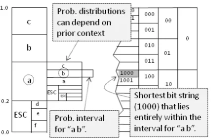
Figure 4: Arithmetic coding.
important that the decompressor exactly recapitu-late the same sequence of Huffman trees that the compressor made. It can do this by counting char-acters as it outputs them, just as the compressor counted characters as it consumed them.
Adaptive compression can also nicely accom-modate shifting topics in text, if we give higher counts to recent events. By its single-pass nature, it is also good for streaming data.
Arithmetic coding. Huffman coding exploits a predictive unigram distribution over the next character. If we use more context, we can make sharper distributions. An n-gram table is one way to map contexts onto predictions.
How do we convert good predictions into good compression? The solution is called arithmetic coding(Rissanen and Langdon Jr., 1981; Witten et al., 1987). Figure 4 sketches the technique. We produce context-dependent probability inter-vals, and each time we observe a character, we move to its interval. Our working interval be-comes smaller and smaller, but the better our pre-dictions, the wider it stays. A document’s com-pression is the shortest bit string that fits inside the final interval. In practice, we do the bit-coding as we navigate probability intervals.
Arithmetic coding separates modeling and com-pression, making our job similar to language mod-eling, where we use try to use context to predict the next symbol.
3.1 PPM
PPM is the most well-known adaptive, predic-tive compression technique (Cleary and Witten, 1984). PPM updates character n-gram tables (usu-ally n=1..5) as it compresses. In a given context, an n-gram table may predict only a subset of char-acters, so PPM reserves some probability mass for
an escape (ESC), after which it executes a hard backoff to the (n-1)-gram table. In PPMA, P(ESC) is 1/(1+D), where D is the number of times the context has been seen. PPMB uses q/D, where q is the number of distinct character types seen in the context. PPMC uses q/(q+D), aka Witten-Bell. PPMD uses q/2D.
PPM* uses the shortest previously-seen deter-ministic context, which may be quite long. If there is no deterministic context, PPM* goes to the longest matching context and starts PPMD. In-stead of the longest context, PPMZ rates all con-texts between lengths 0 and 12 according to each context’s most probable character. PPMZ also im-plements an adaptive P(ESC) that combines text length, number of previous ESC in the con-text, etc.
We use our own C++ implementation of PPMC for monolingual compression experiments in this paper. When we pass over a set of characters in favor of ESC, we remove those characters from the hard backoff.
3.2 PAQ
PAQ (Mahoney, 2005) is a family of state-of-the-art compression algorithms and a perennial Hutter Prize winner. PAQ combines hundreds of mod-els with a logistic unit when making a prediction. This is most efficient when predictions are at the bit-level instead of the character-level. The unit’s model weights are adaptively updated by:
wi ←wi+ηxi(correct−P(1)), where xi =ln(Pi(1)/(1−Pi(1))
η= fixed learning rate
Pi(1)=ith model’s prediction
PAQ models include a character n-gram model that adapts to recent text, a unigram word model (where word is defined as a subsequence of char-acters with ASCII>32), a bigram model, and a skip-bigram model.
4 Bilingual Compression: Prior Work
Nevill and Bell (1992) introduce the concept but actually carry out experiments on paraphrase cor-pora, such as different English versions of the Bible.
without counting the cost of auxiliary files needed for decompression.
Mart´ınez-Prieto et al. (2009), Adiego et al. (2009), Adiego et al. (2010) rewrite bilingual text by first interleaving source words with their trans-lations, then compressing this sequence of bi-words. S´anchez-Mart´ınez et al. (2012) improve the interleaving scheme and include offsets to enable decompression to reconstruct the original word order. They also compare several character-based and word-character-based compression schemes for biword sequences. On Spanish-English Europarl data, they reach an 18.7% compression rate on word-interleaved text, compared to 20.1% for con-catenated texts, a 7.2% improvement.
Al-Onaizan et al. (1999) study the perplexity of learned translation models, i.e., the probabil-ity assigned to the target corpus given the source corpus. They observed iterative training to im-prove training-set perplexity (as guaranteed) but degrade test-set perplexity. They hypothesized that an increasingly tight, unsmoothed translation dictionary might exclude word translations needed to explain test-set data. Subsequently, research moved to extrinsic evaluation of translation mod-els, in the context of end-to-end machine transla-tion.
Foster et al. (2002) and others have used predic-tion to propose auto-complepredic-tions to speed up hu-man translation. As we have seen, prediction and compression are highly related.
5 Predictive Bilingual Compression
Our algorithm compresses target-languagefile2
while looking at source-languagefile1: % bicompress file2 file1 > file2.exe
To make use of arithmetic coding, we consider the task of predicting the next target character, given the source sentence and target string so far:3
P(ej|f1. . . fl, e1. . . ej−1)
If we are able to accurately predict what a human translator will type next, then we should be able to build a good machine translator. Here is an exam-ple of the task:
Spanish: Pido que hagamos un minuto de silencio. English so far: I should like to ob
3We predictefromfin this paper, reversed from Brown et al. (1993), who predictffrome.
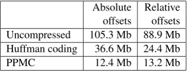
[image:4.595.307.497.62.133.2]Absolute Relative offsets offsets Uncompressed 105.3 Mb 88.9 Mb Huffman coding 36.6 Mb 24.4 Mb PPMC 12.4 Mb 13.2 Mb
Figure 5: Compressing a file of (unidirectional) automatic Viterbi word alignments computed from our large Spanish/English corpus (sentences less than 50 words).
5.1 Word alignment
Let us first work at the word level instead of the character level. If we are predicting the jth English word, and we know that it translates fi
(“aligns to fi”), and if fi has only a handful of
translations, then we may be able to specify ej
with just a few bits. We may therefore suppose that a set of Viterbi word alignments may be useful for compression (Conley and Klein, 2008; S´anchez-Mart´ınez et al., 2012).
We consider unidirectional alignments that link each target position j to a single source position
i(including the null word ati = 0). Such align-ments can be computed automatically using EM (Brown et al., 1993), and stored in one of two for-mats:
Absolute: 1 2 5 5 7 0 3 6 . . .
Relative: +1 +1 +3 0 +2 null -4 +3 . . . In order to interpret the bits produced by the compressor, our decompressormust also have ac-cess to the same Viterbi alignments. Therefore, we must include those alignments at the beginning of the compressed file. So let’s compress them too.
How compressible are alignment sequences? Figure 5 gives results for Viterbi alignments de-rived from our large parallel Spanish/English cor-pus. First, some interesting facts:
• Huffman works better on relative offsets, be-cause the common “+1” gets a short bit code.
• PPMC’s use of context makes it impressively insensitive to alignment format.
• PPMC beats Huffman on relative offsets. This would not happen if relative offset inte-gers were independent of one another, as as-sumed by (Brown et al., 1993) and (Vogel et al., 1996). Bigram statistics bear this out:
P(+1|-2) = 0.20 P(+1|+1) = 0.59 P(+1|-1) = 0.20 P(+1|+2) = 0.49 P(+1|0) = 0.52
suggests that translation aligners might want to model more context than just P(offset).
However, the main point of Figure 5 is that the compressed alignment file requires 12.4 Mb! This is too large for us to prepend to our compressed file, for the sake of enabling decompression.
5.2 Translation dictionary
Another approach is to forget Viterbi alignments and instead exploit a probabilistic translation dic-tionary table t(e|f). To predict the next target wordej, we admit the possibility thatejmight be
translatinganyof the source tokens. IBM Model 2 (Brown et al., 1993) tells us how to do this:
Givenf1. . . fl:
1. Choose English lengthm (m|l) 2. Forj= 1..m, choose alignmentaj a(aj|j, l)
3. Forj= 1..m, choose translationej t(ej|faj)
which, via the “IBM trick” implies: P(e1. . . em|f1. . . fl)=
(m|l)Qm
j=1Pli=0a(i|j, l)t(ej|fi)
In compression, we must predict English words in-crementally, before seeing the whole string. Fur-thermore, we must predict P(ST OP) to end the English sentence. We can adapt IBM Model 2 to make incremental predictions:
P(ST OP|f1. . . fl, e1. . . ej−1)∼ P(ST OP|j, l)=
(j−1|l)/Pmax
k=j−1(k|l) P(ej|f1. . . fl, e1. . . ej−1)∼ P(ej|f1. . . fl)=
[1−P(ST OP|j, l)]Pli=0a(i|j, l)t(ej|fi)
We can traint, a, andon our bilingual text us-ing EM (Brown et al., 1993). However, thet-table is still too large to prepend to the compressed En-glish file.
5.3 Adaptive translation modeling
Instead, inspired by PPM, we build up transla-tion tables in RAM, during a single pass of our compressor. Our decompressor then rebuilds these same tables, in the same way, in order to interpret the compressed bit string.
Neal and Hinton (1998) describe online EM, which updates probability tables after each train-ing example. Liang and Klein (2009) and Leven-berg et al. (2010) apply online EM to a number of language tasks, including word alignment. Here we concentrate on the single-pass case.
We initialize a uniform translation model, use it to collect fractional counts from the first segment
pair, normalize those counts to probabilities, use those new probabilities to collect fractional counts from the second segment pair, and so on. Because we pass through the data only once, we hope to converge quickly to high-quality tables for com-pressing the bulk of the text.
Unlike in batch EM, we need not keep sepa-rate count and probability tables. We only need count tables, including summary counts for nor-malization groups, so memory savings are signif-icant. Whenever we need a probability, we com-pute it on the fly. To avoid zeroes being immedi-ately locked in, we invoke add-λsmoothing every time we compute a probability from counts:4
t(e|f) = count(e,f)+λt
count(f)+λt|VE|
a(i|j, l) = count(i,j,l)+λa
count(j,l)+λa(l+1)
where|VE|is the size of the English vocabulary.
We determine|VE|via a quick initial pass through
the data, then include it at the top of our com-pressed file.
In batch EM, we usually run IBM Model 1 for a few iterations before Model 2, gripped by an atavistic fear that theaprobabilities will enforce rigid alignments before word co-occurrences have a chance to settle in. It turns out this fear is jus-tified in online EM! Because the atable initially learns to align most words to null, we smooth it more heavily (λa= 102,λt= 10−4).
We also implement a single-pass HMM align-ment model (Vogel et al., 1996). In the IBM mod-els, we can either collect fractional counts after we have compressed a whole sentence, or we can do it word-by-word. In the HMM model, alignment choices are no longer independent of one another:
Givenf1. . . fl:
1. Choose English lengthmw/prob(m|l)
2. Forj= 1..m:
2a. setajto null w/probp1,or
2b. choose non-nullajw/prob(1−p1)o(aj−ak)
3. Forj= 1..m, choose translationejw/probt(ej|faj) In the expression o(aj −ak), k is the maximum
English index (k < j) such that ak 6= 0. The
relative offseto-table learns to encourage adjacent English words to align to adjacent Spanish words. Batch HMM performs poorly under uniform initialization, with two causes of failure. First, EM training setso(0)too high, leading to absolute alignments like “1 2 2 2 5 5 5 5 . . . ”. We avoid
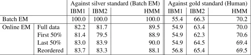
Against silver standard (Batch EM) Against gold standard (Human)
IBM1 IBM2 HMM IBM1 IBM2 HMM
Batch EM 100.0 100.0 100.0 55.4 66.3 70.2
Online EM Full data 82.2 81.7 89.5 54.9 63.4 70.0
First 50% 81.4 79.5 88.9 54.9 62.3 70.6
Last 50% 83.0 83.9 90.0 54.9 64.5 69.4
Reordered 83.7 83.3 88.1 56.8 65.4 69.5
Figure 6: Word alignment f-scores. Batch EM for IBM 1 is run for 5 iterations; Batch IBM2 adds 5 further iterations of IBM2; Batch HMM adds a further 5 iterations of HMM. Online EM is single-pass. Against the silver standard, alignments are unidirectional; against gold, they are bidirectional and symmetrized with grow-dial-final (Koehn et al., 2003). First and last 50% report on different portions of the corpus. Reordered is on segment pairs ordered short to long. All runs exclude segment pairs with segments longer than 50 words.
this with a standard schedule of 5 IBM1 iterations, 5 IBM2 iterations, then 5 HMM iterations. How-ever, HMM still learns a very high value for p1, aligning most tokens to null, so we fix p1 = 0.1 for the duration of training.
Single-pass, online HMM suffers the same two problems, both solved when we smooth differen-tially (λo= 102, λt= 10−4) and fixp1 = 0.1.
Two quick asides before we examine the effec-tiveness of our online methods:
• Translation researchers often drop long seg-ment pairs that slow down HMM model pro-cessing. In compression, we cannot drop any of the text. Therefore, if the source segment contains more than 50 words, we use only monolingual PPMC to compress the target. This affects 26.5% of our word tokens.
• We might assist an online aligner by permut-ing ournsegment pairs to place shorter, less ambiguous ones at the top. However, we would have to communicate the permutation to the decompressor, at a prohibitive cost of log2(n!)/(8·106)= 4.8 Mb.
We next look at alignment accuracy (f-score) on our large Spanish/English corpus (Figure 6). We evaluate against both a silver standard (Batch EM Viterbi alignments5) and a gold standard of 334 human-aligned segment pairs distributed through-out the corpus. We see that online methods gener-ate competitive translation dictionaries. Because single-pass alignment is significantly faster than traditional multi-pass, we also investigate its im-pact on an overall Moses pipeline for phrase-based
5We confirm that our Batch HMM implementation gives f-scores (f=70.2, p=80.4, r=62.3) similar to GIZA++ (f=71.2, p=85.5, r=61.0), and its differently parameterized HMM.
Alignment Test Set Bleu speed Europarl News Batch HMM 1230.78 min 30.2 26.2 Online HMM 711.87 min 30.0 25.3
Figure 7: Fast, single-pass HMM alignment yields competitive Spanish-English Moses phrase-based translation accuracy, as measured by Bleu (Papineni et al., 2002). In-domain (Europarl) and out-of-domain (SMAT-07 News Commen-tary) tune/test sets each consist of approximately 1000 sentences, all longer than 50 words to avoid overlap with training.
machine translation (Koehn et al., 2007). Figure 7 shows that we can achieve competitive translation accuracy using fast, single-pass alignment, speed-ing up the system development cycle. For this use case, we can get an additional +0.3 alignment f-score (just as fast) if we print Viterbi alignments in a second pass instead of during training.
5.4 Word tokenization
We now want our continuously-improving trans-lation model (TM) to predict target text, and to combine its predictions with PPM’s. For that to happen, our TM will need to predict the exact text, including spurious double-spaces, how parenthe-ses combine with quotation marks, and so on.
[image:6.595.74.509.63.159.2]recoverability intact. Finally, we move any suffix on an alpha-numeric wordito become a prefix on a non-alpha-numeric wordi+ 1. This reduces the vocabulary size for TM learning. An example:
"String-theory?" he asked. <=>
S@0 "@0 String@0 -@0 theory@0 ?@0 "@1 he@2 asked@0 .@0
<=>
S@0 "@0 String@0 -@0 theory@0 ?@0 " he@2 asked@0 .@0
<=>
S@0 "@0 String @0-@0 theory @0?@0 " he@2 asked @0.@0
5.5 Predicting target words
Under this tokenization scheme, we now ask our TM to give us a probability distribution over pos-sible next words. The TM knows the entire source word sequencef1...fland the target words e1...ej−1 seen so far. As candidates, we consider target words that can be produced, via the current t-table, from any (non-NULL) source words with probability greater than10−4.
For HMM, we compute a prediction lattice that gives a distribution over possiblesource alignment positions for the current word we are predicting. Intuitively, the prediction lattice tells us “where we currently are” in translating the source string, and it prefers translations of source words in that vicin-ity. We efficiently reuse the lattice as we make predictions for each subsequent target word.
To make the TM’s prediction more accurate, we weight its prediction for each word with a smoothed, adapted English bigram word language model (LM). This discourages the TM from trying to predict the first character of a word by simply using the most frequent source words. We found that exponentiating the LM’s score by 0.2 before weighting keeps it from overpowering the HMM predictions.
5.6 Predicting target characters
To convert word predictions into character predic-tions, we combine scores for words that share the next character. For example, if the TM predicts ”monkey 0.4, car 0.3, cat 0.2, dog 0.1”, then we have ”P(c) 0.5, P(m) 0.4, P(d) 0.1”. Addition-ally, we restrict ourselves to words prefixed by the portion ofej already observed. The TM predicts
the space character when a predicted word fully matches the observed prefix.
We also adjust PPM to produce a full distribu-tion over the 96 possible next characters. PPM
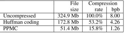
File Compression size rate bpb Uncompressed 324.9 Mb 100.0% 8.00 Huffman coding 172.8 Mb 53.2% 4.26
[image:7.595.308.513.62.116.2]PPMC 51.4 Mb 15.8% 1.26
Figure 8: Compression of the Spanish side of the bilingual corpus. bpb = bits per byte.
File Compression size rate bpb Uncompressed 294.5 Mb 100.0% 8.00 Huffman coding 160.7 Mb 54.6% 4.37
PPMC 48.5 Mb 16.5% 1.32
Bilingual (this paper) 35.0 Mb 11.9 % 0.95
Shannon monolingual 1.61
[image:7.595.308.516.161.248.2]Shannon bilingual 0.51
Figure 9: Main results. Compression of the En-glish side of the bilingual corpus. Bilingual com-pression improves results. For Shannon game studies, bpb are estimated as cross-entropies of n-gram models fitted to human guess sequences.
normally computes a distribution over only char-acters previously seen in the current context (plus ESC). We now back off to the lowest context for every prediction.
We interpolate PPM and TM probabilities: P(ek|f1. . . fl, e1. . . ek−1)=
µPP P M(ek|e1. . . ek−1)+
(1−µ)PT M(ek|f1. . . fl, e1. . . ek−1) We adjustµdynamically based on the relative con-fidence of the models:
µ
=
max(P P Mmax(P P M))2.5+max(HMM2.5 )2.5 Here,max(model)refers to the highest probabil-ity assigned to any character in the current context by the model. This yields better compression rates than simply settingµto a constant. When the TM is unable to extend a word, we setµ= 1.6 Results
Figure 8 shows that monolingual PPM compresses the Spanish side of our corpus to 15.8% of the original. Figure 9(Main results)shows results for the English side of the corpus. Monolingual PPM compresses to 16.5%, while our HMM-based bilingual compression compresses to 11.9%.6
We can say that a human translation is charac-terized by an additional 0.95 bits per byte on top of the original, rather than the 1.32 bits per byte we
File Compression size rate bpb Uncompressed 619.4 Mb 100.0% 8.00 Huffman coding 336.8 Mb 54.4% 4.35
PPMC 101.6 Mb 16.4% 1.31
Bilingual (this paper) 86.4 Mb 13.9% 1.12 (S´anchez-Mart´ınez different 20.1% 1.61 et al., 2012) PPMDI corpus
[image:8.595.72.280.62.169.2](S´anchez-Mart´ınez different 18.7% 1.50 et al., 2012) bilingual corpus
Figure 10: Compression of Spanish plus English. All methods are run on a single file of Spanish concatenated with English, except for “Bilingual (this paper),” which records the sum of (1) Span-ish compression and (2) EnglSpan-ish-given-SpanSpan-ish compression. Comparative numbers copied from S´anchez-Mart´ınez et al (2012) are for a different subset of Europarl data.
would need if the English were independent text. Assuming our Spanish compression is good, we can also say that the human translator produces at most 68.1% (35.0/51.4) of the information that the original Spanish author produced. Intuitively, we feel this bound is high and should be reduced with better translation modeling.
Figure 9 also reports our Shannon game exper-iments in which bilingual humans guessed subse-quent characters of the English text. As suggested by Shannon, we upper-bound bpb as the cross-entropy of a unigram model over a human guess sequence(e.g., 1 1 2 5 17 1 1 . . . ), which records how many guesses it took to identify each subse-quent English character, given context. For a 502-character English sequence, a team of four bilin-guals working together gave us an upper-bound bpb of 0.51. This team had access to the original Spanish, plus a Google translation. Monolinguals guessing on the same data (minus the Spanish and Google translation) yielded an upper-bound bpb of 1.61. These human-level models indicate that hu-man translators are actually only adding ∼ 32%
more information on top of the original, and that our current translation models are only capturing some fraction of this redundancy.7
Figure 10 shows compression of the entire bilingual corpus, allowing us to compare with the previous state-of-the-art (S´anchez-Mart´ınez et al., 2012), which compresses a single, word-interleaved bilingual corpus. It shows how PPMC
7Machine models can also generate guess sequences, and we see that entropy of a 30m-character PPMC guess sequence (1.43) upper-bounds actual PPMC bpb (1.28).
does on a concatenated Spanish/English file. Uncompressed English (294.5 Mb) is 90.6% the size of uncompressed Spanish (324.9 Mb). Huff-man narrows this gap to 93.0%, and PPM nar-rows it further to 94.4%, consistent with Behr et al. (2003) and Liberman (2008). Spanish redun-dancies like adjective-noun agreement and bal-anced question marks (“¿ . . . ?”) may remain un-exploited.
7 Conclusion
We have created a bilingual text compression chal-lenge web site.8 This web site contains standard bilingual data, specifies what a valid compression is, and maintains benchmark results.
There are many future directions to pursue. First, we would like to develop and exploit better predictive translation modeling. We have so far adapted machine translation technology circa only 1996. For example, the HMM alignment model cannot “cross off” a source word and stop trying to translate it. Also possible are phrase-based trans-lation, neural nets, or as-yet-unanticipated pattern-finding algorithms. We only require an executable that prints the bilingual text.
Our current method requires segment-aligned input. To work with real-life bilingual corpora, the compressor should take care of segment align-ment, in a way that allows decompression back to the original text. Similarly, we are currently re-stricted to texts written in the Latin alphabet, per our definition of “word.”
More broadly, we would also like to import more compression ideas into NLP. Compression has so far appeared sporadically in NLP tasks like native language ID (Bobicev, 2013), text in-put methods (Powers and Huang, 2004), word segmentation (Teahan et al., 2000; Sornil and Chaiwanarom, 2004; Hutchens and Alder, 1998), alignment (Liu et al., 2014), and text categoriza-tion (Caruana & Lang, unpub. 1995).
Translation researchers may also view bilingual compression as an alternate, reference-free evalu-ation metric for translevalu-ation models. We anticipate that future ideas from bilingual compression can be brought back into translation. Like Brown et al. (1992), with their gauntlet thrown down and
fury of competitive energy, we hope that cross-fertilizing compression and translation will bring fresh ideas to both areas.
Acknowledgements
This work was supported by a USC Provost Fel-lowship and ARO grant W911NF-10-1-0533.
References
Joaqu´ın Adiego, Nieves R. Brisaboa, Miguel A. Mart´ınez-Prieto, and Felipe S´anchez-Mart´ınez. 2009. A two-level structure for compressing aligned bitexts. In String Processing and Information Re-trieval. Springer-Verlag.
Joaqu´ın Adiego, Miguel A. Mart´ınez-Prieto, Javier E. Hoyos-Tor´ıo, and Felipe S´anchez-Mart´ınez. 2010. Modelling parallel texts for boosting compression. InProc. Data Compression Conference (DCC). Yaser Al-Onaizan, Jan Curin, Michael Jahr, Kevin
Knight, John Lafferty, Dan Melamed, Franz-Josef Och, David Purdy, Noah A. Smith, and David Yarowsky. 1999. Statistical machine translation. Technical Report http://bit.ly/1u9jJsx, Johns Hop-kins University.
F. Behr, Victoria Fossum, Michael Mitzenmacher, and David Xiao. 2003. Estimating and comparing en-tropies across written natural languages using PPM compression. InProc. Data Compression Confer-ence (DCC).
Victoria Bobicev. 2013. Native language identification with PPM. InProc. NAACL.
Peter F. Brown, Vincent J. Della Pietra, Robert L. Mer-cer, Stephen A Della Pietra, and Jennifer C. Lai. 1992. An estimate of an upper bound for the entropy of English. Computational Linguistics, 18(1):31– 40.
Peter F. Brown, Vincent J. Della Pietra, Stephen A. Della Pietra, and Robert L. Mercer. 1993. The mathematics of statistical machine translation: Parameter estimation. Computational linguistics, 19(2):263–311.
John G. Cleary and Ian Witten. 1984. Data com-pression using adaptive coding and partial string matching. IEEE Transactions on Communications, 32(4):396–402.
Ehud S. Conley and Shmuel T. Klein. 2008. Using alignment for multilingual text compression. Inter-national Journal of Foundations of Computer Sci-ence, 19(01):89–101.
Ehud S. Conley and Shmuel T. Klein. 2013. Im-proved alignment-based algorithm for multilingual text compression. Mathematics in Computer Sci-ence, 7(2):137–153.
George Foster, Philippe Langlais, and Guy Lapalme. 2002. User-friendly text prediction for translators. InProc. EMNLP.
David A. Huffman et al. 1952. A method for the con-struction of minimum redundancy codes. Proc. IRE, 40(9):1098–1101.
Jason L. Hutchens and Michael D Alder. 1998. Find-ing structure via compression. InProc. Joint Con-ferences on New Methods in Language Processing and Computational Natural Language Learning. Marcus Hutter. 2006. 50,000 Euro prize for
com-pressing human knowledge. http://prize. hutter1.net. Accessed: 2015-02-04.
Philipp Koehn, Franz Josef Och, and Daniel Marcu. 2003. Statistical phrase-based translation. InProc. NAACL.
Philipp Koehn, Hieu Hoang, Alexandra Birch, Chris Callison-Burch, Marcello Federico, Nicola Bertoldi, Brooke Cowan, Wade Shen, Christine Moran, Richard Zens, et al. 2007. Moses: Open source toolkit for statistical machine translation. InProc. ACL Poster and Demo Session.
Philipp Koehn. 2005. Europarl: A parallel corpus for statistical machine translation. InProc. MT Summit X.
Patrik Lambert, Adri`a De Gispert, Rafael Banchs, and Jos´e B Mari˜no. 2005. Guidelines for word align-ment evaluation and manual alignalign-ment. Language Resources and Evaluation, 39.
Abby Levenberg, Chris Callison-Burch, and Miles Os-borne. 2010. Stream-based translation models for statistical machine translation. In Proc. NAACL, pages 394–402. Association for Computational Lin-guistics.
Percy Liang and Dan Klein. 2009. Online EM for un-supervised models. InProc. HLT-NAACL.
Mark Liberman. 2008. Is English more efficient than Chinese after all? http://languagelog. ldc.upenn.edu/nll/?p=93. Accessed: 2015-02-04.
Wei Liu, Zhipeng Chang, and William J. Teahan. 2014. Experiments with a PPM compression-based method for English-Chinese bilingual sen-tence alignment. InStatistical Language and Speech Processing, pages 70–81. Springer.
M. V. Mahoney. 2005. Adaptive weighting of context models for lossless data compression. Technical Re-port CS-2005-16, Florida Institute of Technology. M. A. Mart´ınez-Prieto, J. Adiego, F.
S´anchez-Mart´ınez, P. de la Fuente, and R. C. Carrasco. 2009. On the use of word alignments to enhance bitext compression. InProc. Data Compression Confer-ence (DCC).
Craig Nevill and Timothy Bell. 1992. Compression of parallel texts. Information Processing & Manage-ment, 28(6):781–793.
Kishore Papineni, Salim Roukos, Todd Ward, and Wei-Jing Zhu. 2002. Bleu: a method for automatic eval-uation of machine translation. InProc. ACL. David Martin Powers and Jin Hu Huang. 2004.
Adap-tive compression-based approach for chinese pinyin input. InProc. Third SIGHAN Workshop on Chinese Language Learning.
Jorma Rissanen and Glen G Langdon Jr. 1981. Univer-sal modeling and coding.Information Theory, IEEE Transactions on, 27(1):12–23.
Felipe S´anchez-Mart´ınez, Rafael C. Carrasco, Miguel A. Mart´ınez-Prieto, and Joaquin Adiego. 2012. Generalized biwords for bitext compression and translation spotting. Journal of Artificial Intelligence Research, 43:389–418.
Ohm Sornil and Paweena Chaiwanarom. 2004. Com-bining prediction by partial matching and logistic re-gression for thai word segmentation. InProc. COL-ING, page 1208. Association for Computational Lin-guistics.
William John Teahan, Yingying Wen, Rodger McNab, and Ian H. Witten. 2000. A compression-based al-gorithm for Chinese word segmentation. Computa-tional Linguistics, 26(3):375–393.
Stephan Vogel, Hermann Ney, and Christoph Tillmann. 1996. HMM-based word alignment in statistical translation. InProc. COLING.