Computing worst case execution time (WCET) by Symbolically Executing a time-accurate Hardware Model

Computing worst case execution time (WCET) by

Symbolically Executing a time-accurate Hardware Model

Bilel Benhamamouch, Bruno Monsuez

∗

Abstract—To ensure that a program will respect all its tim-ing constraints we must be able to compute a safe estimation of its worst case execution time (WCET). However with the increas-ing sophistication of the processors, computincreas-ing a precise estima-tion of the WCET becomes very difficult. In this paper, we pro-pose a novel formal method to compute a precise estimation of the WCET that can be easily parameterized by the hardware ar-chitecture. Assuming that there exists an executable timed model of the hardware, we first use symbolic execution [1] to precisely infer the execution time for a given instruction flow. Then we merge the states relying on the loss of precision we are ready to accept.

Keywords: static analysis, WCET, processor modelization, symbolic execution.

1

Introduction

Computing WCET is useful either to determine appropriate scheduling schemes for the tasks or to perform an overall schedulability analysis. This is done obviously in order to guarantee that all timing constraints will be met. Computing program execution time has always been difficult. Dynamic methods [11, 12] as well as formal methods [5, 8] have re-ceived a lot of attention for precise estimation of the worst case execution time of code snippets. However, current meth-ods have some difficulties to cope with the increasing com-plexity of the hardware used to implement critical real time applications.

In this paper, we present part of our formal method [15] to compute an upper estimation of the WCET that contains the loss of precision and that can also be parameterized by current complex hardware architecture like super-scalar microproces-sor or multi-procesmicroproces-sor systems.

The contribution of this paper is twofold, on one hand we show how easily we abstract the behavior of a current hardware ar-chitecture in order to highlight its timing properties, and on the other we propose an approach which uses this abstraction to compute the WCET of a sequence of code.

The paper is organized as follows: we first present how the formal methods which are usually used to compute WCET (Section 2) and we give an overview of our framework (Sec-tion 3). Then, we show how we compute the execu(Sec-tion time of an instruction sequence using symbolic execution as well

∗_{Ecole Nationale Supérieure de Techniques Avancées UEI, ENSTA 32}

Bd Victor, 75739 Paris cedex 15, France [email protected], [email protected]

as how we abstract the executable timed model to manage the explosion of the states generated by the symbolic execution (Section 4). After that, we illustrate our approach through an example (Section 5). In Section 6, we give an overview of how the merging policy works. Finally, we conclude and we present ongoing and future works (Section 7).

2

Formal methods

Nowadays the most mature method which allows to compute an over approximation of the WCET is the one developed by AbsInt team. This method can be described as follow: Initially, a control flow graph (CFG) is extracted from the bi-nary code. Then on this CFG a value analysis is carried out to produce an approximation (intervals) of the memory ar-eas which will be reached. This result is in turn exploited by the following stage represented by the cache analysis which is used to classify the memory references in:

• Cache always hit: The memory reference always results in a cache hit.

• Cache always miss: The memory reference always re-sults in a cache miss.

• Persist: The referenced memory block will be load at most once.

• Not classified: The memory reference could not be clas-sified in one of the above groups.

When this classification is made for all blocks, it is injected as input of the following analysis. This will define the possible states of the pipeline at each execution point of the analyzed program. Therefore, it will be associated to each instruction various execution times (each one is related to a precise envi-ronment). At this moment it is useful to specify that the im-plementation of these various analyses was possible because it is based on abstract interpretation [9, 10]. This technique is largely used for program checking, and it makes possible to associate concrete values to abstract ones (a whole of con-crete values could thus be represented by an abstract value). The various results obtained during the preceding stages, are finally exploited jointly with the source code by the last anal-ysis called path analanal-ysis. This analanal-ysis is based on linear pro-gramming techniques. That enables it to produce the longest execution path.

This approach is represented by a sequential analysis formed by black boxes [5, 8]. This is one of the strong points of this approach, considering that it makes possible to use different

techniques at various levels of the study, such as: using ab-stract interpretation for the cache and the pipeline analysis, while the path analysis is done by ILP (integer linear program-ming). But this strength can also be a weakness [6, 7]. Indeed, the increase in complexity of the hardware platform leads to an increase in the number of black boxes required to perform the analysis as well as a more complex design for each black box that abstracts the hardware semantics.

In addition, those formal methods have three main drawbacks. During the analysis the dependencies between the black boxes cannot be identified precisely which leads those methods to explore a superset of all execution paths. Thus WCETs for un-feasible execution paths are taken into account (1); To avoid the state explosion, execution paths are merged using tools provided by abstract interpretation like widening operator, that may also conducts to an over-exaggerated approximation of the execution time (2); The analyzer must explicitly support the target platform and must provide valuable abstraction of the hardware components that compose the target platform (3).

3

Our framework

Our approach is mainly based on the symbolic execution. So before explaining how the method works let us describe what is the symbolic execution.

3.1

Background: Symbolic execution

The main idea behind symbolic execution [1, 2] is to use sym-bolic values instead of actual data to represent the input val-ues. As a result, the output values computed by a program are expressed as a function of symbolic values. Evaluation of assignments is done naturally, the left-hand side variable re-ceives the resulting symbolic expression, which should be a polynomial.

Evaluation of alternatives is a bit more complicated. It re-quires that a "path condition"PC– a Boolean expression over the symbolic inputs – is added to the execution state. The path conditionPC is a (quantifier-free) boolean formula over the symbolic inputs; it accumulates constraints which the inputs must satisfy in order for an execution to follow the particular associated execution path. At program start, each symbolic execution begins withPCinitialized to true. When encoun-tering an alternative, evaluation first starts with the evaluation of the associated Boolean expression by replacing variables by their values. Since the values of variables are polynomials over the symbols, the condition is an expression of the form:

P > 0, whereP is a polynomial. Call such an expression R. Then we can have three cases:

• PC ⊃ R and PC 6⊃ ¬R: The expression is always true, the execution continues with the conditional code sequence.

• PC⊃ ¬RandPC6⊃R: The expression is always false, the execution continues with the "else" code sequence if an "else" block is available or simply ignore the condi-tional code sequence.

• Otherwise, the Boolean condition may be true or false. In this case, we split the path condition in two paths con-ditionsPC_true = PC∧RandPC_false =PC∧ ¬R. We continue the concurrent execution of the condition code sequence withPC_trueand the "else" code sequence or the code located after the conditional code sequence with the path conditionPC_false.

3.2

Conjoint symbolic execution of binary code and

time-accurate system model

To mitigate the drawbacks of the formal methods (section II), we propose a new approach that extends the classical frame-works for computing the worst case execution time of a se-quence of code with no loops or branch instruction. This new framework provides two main advantages over the methods currently used: (1) it simply requires an executable timed-model of the target platform and does not require the design of black boxes that abstract the hardware semantics, this is achieved by the conjoint symbolic execution of the program code and the executable model of the processor, (2) it pro-vides a method that allows to identify execution states that can be merged with no loss of precision as well as gives insight in the resulting loss of precision when merging execution paths that have similar but different execution times, this is achieved by the backward execution paths merging with symbolic exe-cution lookup policy.

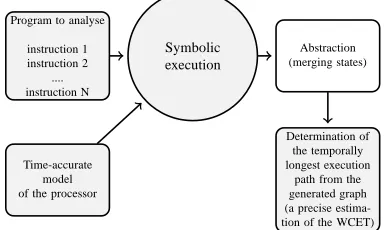
In this paper, we focus on the conjoint symbolic execution part of the analysis method. During symbolic program execution, the executable model of the processor is used to compute for each execution point all the states that the processor may reach when executing this instruction with respect to the execution history. Following this reasoning we build a symbolic tree which contains:

(1) All the states that the processor may reach during the exe-cution (only the possible paths are taken into account). (2) The transitions are labeled with the maximum number of clock cycles needed to move from one state to another. So at the end of the analysis, we easily extract from the tree the temporally longest execution path. In the next section

(Sec-Program to analyse

instruction 1 instruction 2

.... instruction N

Symbolic execution

Abstraction (merging states)

Time-accurate model of the processor

Determination of the temporally longest execution

[image:2.612.326.518.507.622.2]

path from the generated graph (a precise estima-tion of the WCET)

Figure 1: WCET estimation method

tion 4), we explain how we build a symbolic tree which con-tains all the possible execution times of the analyzed program as well as how we abstract it in order to reduce the number of the generated states whithout introducing any loss of pre-cision. Then, we present some significant architectural details

of the hardware used in our framework as well as a small pro-gram to illustrate our approach (Section 5). Finally, we give in section 6 an overview of how the merging policy works.

4

Using an executable timed-model of the

tar-get system to Compute the WCET

4.1

An executable timed model of the target

archi-tecture

During our analysis we must provide an executable timed model of the hardware. This abstract timed model is first mod-eled in C++ with some SystemC facilities. Further extensions could accept full SystemC TLM-T, SystemC Verilog, VHDL or Verilog descriptions.

The executable timed model Basically a processor can be

seen as a complex component which is composed by several units. Each one carries out a number of tasks during a clock cycle. The current processor state is the product of the states of all the basic units of the processor.

Definition 1 System unit states & system states A system unit

stateSC[u]is a minimal set of properties that allows to define what is the next operation that this unituwill perform. The state of the target system SC is the product of all the states of the units that compose this system SC: SC = (⊗uunit ofSSC[u]).

4.2

Building a symbolic graph

The state s of a symbolically executed binary program in-cludes the system state SC the processor state (pipeline, data/instruction cache and thePC), andSVthe symbolic val-ues. The executable timed model is symbolically executed for the given program. This model takes as an input a current state

SCof the system and returns the processor statesSC0

obtained after executing the model during one clock cycle.

We begin the symbolic execution of the code snippet with an empty pipeline(P=empty)1_{and no information about the}

cache states(IC=DC=>).

Starting from this initial state and relying on the processor de-scription we execute the code symbolically. So, we compute on each clock cycle the set of next states. This set contains all the states that the processor may reach when it starts ex-ecuting the code with respect to the execution history. For instance, after each cache miss the processor initiates a mem-ory transaction that loads a cache line. If during the execution a cache miss occurs when accessing a word, the cache gets up-dated. So accessing the double word that follows immediately the loaded word will result in a cache hit.

4.3

Simplifying the generated symbolic graph

The model of the target architecture must be timed, that means that it must preserve the time (number of clock cycles) the

1_{This assumption is made because starting an execution with an unknown}

pipeline state implies having some information about the running application, which implies other assumptions.

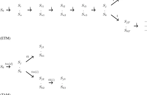
processor needs to execute an instruction. The simplest im-plementation of timed model use the clock as the base cycle. So for each clock cycle, it computes the new state of the pro-cessor. However, in the presence of cache misses and pipeline stalls, it may lead to unnecessary intermediate states, since the processor is waiting for some data. A more efficient imple-mentation is the time-accurate model, as shown on figure 2. It is achieved when returning the next processor state that is different from the current one as well as the number of clock cycles required to reach this processor state.

Definition 2 Clock-accurate model & Time-accurate model

An executable clock-accurate model is an executable function that maps a system state SC to the next system stateSC0 at the next clock cycle. An executable time-accurate model is an executable function that maps a system stateSCto the pair of a system state SC0

and the timet ∈ T needed to reach this system state.

The atomic times that are associated to a particular cache op-eration are:

th: time associated to a cache hit. tm: time associated to a cache miss.

trl: time associated to a cache line reloading. (d): data cache. (i): instruction cache.

During the execution data and instruction caches are ab-stracted to indicate the state of the cache (busy or idle) as well as to tell if the requested data is present in the cache.

4.4

Symbolic execution of the time-accurate model

As described before, the time-accurate model takes as an input a current stateSCof the system and returns the next processor stateSC0

that is different from the current one as well as the number of clock cycles required to reach this system state. Symbolic execution of the time-accurate model takes as an entry the current symbolic statesof the system and returns a set final states as well as the respective times required to reach this final states:{(s1, t1), . . . ,(sn, tn)}.

Definition 3 Intermediate states If s ∈ S is a valid

sys-tem state, we call “intermediate states” the final states {(s1, t1), . . . ,(sn, tn)}generated by one step of symbolic

exe-cution of the time-accurate model when starting the exeexe-cution with the states.

Definition 4 Timed Symbolic Execution Graph The

sym-bolic execution graph(N,TR,M)is a graph that describes the symbolic execution of a code sequence and is defined as follow:

• the nodesN of the graphs are symbolic states,

• the transitions TR: (N × N)map a nodeN to another nodeN.

• the labeling functionMmaps TR−→ T and associates to each transition tr = (ns×ne)the number of clock

cycles that the system takes to go from the starting state

nsto the ending stateneof the transition.

Now, we present the algorithm that builds the timed symbolic execution tree for a sequence of binary instructions.

Sj1

.

Sk1

S0 Si

.

Sn

Si1

.

Sn1 Si2

.

Sn2 Si3

.

Sn3 Sj

.

Sk

Sj20

.

Sk20

... ... ...

(ETM)

Sj1

.

Sk1

S0 Sj

.

Sk

Sj2

.

Sk2

Sj3

.

Sk3

(TAM)

1 1 1 1 1

1 1

1

tm(d)

th

tm(i)

[image:4.612.54.293.48.203.2]

th(i)

Figure 2: Symbolic execution of the executable timed (ETM) and the time-accurate model (TAM)

r← {initial processor state (pipeline & data cache),PC

=true}, ; // Initialization

current_states← {r},G ← {r};

whilecurrent_statesis not empty do //

Propagation

Removes statesfromcurrent_states; Computes the symbolic successors

{(ss

1, t1), . . . ,(ssn, tn)}ofs;

Adds all transitionss−→ti _ss

i to the symbolic

execution graphG;

Adds to the setcurrent_statesall the statesss i

that are not terminal states (terminal states are the final states generated by the last instruction of the code sequence);

5

Framework’s illustration

In this section we propose a description of a hardware archi-tecture in order to show how we abstract this description and how we use the resulting abstraction to compute a precise es-timation of the WCET. Before starting the processor’s mod-elization, we should decide about the characteristics that we will need during the analysis. These characteristics represent, on each clock cycle, not only the state of the processor but also allow to identify precisely what are the reachable states on the next clock cycle.

5.1

Processor’s description

To build the processor state, first we can imagine that a combi-nation of the pipeline and the cache states will suffice to have a precise representation of the hardware. However, during the analysis, relying on this representation we cannot identify pre-cisely the next reachable states. To solve this problem, the pro-cessor’s state must be enriched with a "path condition (PC)" (Section 3). This PC provides to identify at each execution point of the control flow graph which path should be taken. So we represent a processor state by a combination of:

(1) a pipeline state (see below the definition).

(2) cache state (instruction and data): it is represented by the instruction (or data) that it contains.

(3) a PC: as seen in section 3, it accumulates constraints which the inputs must satisfy in order for an execution to follow the particular associated execution path.

Now we will focus on describing the pipeline state. Note that most of the pipelines developed in order to be integrated into an embedded system contain at least :

Fetch: On each clock cycle, this unit retrieves instruction(s)

from the memory system and computes the location of the next instruction(s).

Dispatch: This unit decodes the instructions supplied by the

instruction fetch stage and dispatches them to the appropriate execution unit.

Execute: Each execution unit that has an executable

instruc-tion executes the selected instrucinstruc-tion, and notifies the comple-tion stage that the instruccomple-tion has finished execucomple-tion. Nowa-days, most of the pipelines integrate at least five execution units : an integer unit (IU), a floating-point unit (FPU), a branch processing unit (BPU), a load/store unit (LSU), and a system register unit (SRU).

Complete/writeback: This pipeline stage maintains the

cor-rect architectural machine state and transfers the results to the appropriate registers as instructions are retired.

The following table summarizes the pipeline stages.

Processor units

F: Fetcher CU: Completion Unit

D: Dispatcher SRU: System Register Unit LSU: Load Store Unit RS: Reservation Station IU: Integer Unit FPU: Float Point Unit BPU: Branch Processing Unit

During the execution the states of the units are characterized by the instructions that are currently executed (eg. IU2 indi-cates that the integer unit executes the second instruction of the program).

5.2

Processor’s modelization

Before starting the analysis we must provide a model of the processor. it is a simple program (see figure 3 which repre-sents the fetch Unit) that describes the processor’s behavior. The processor’s model works as follow: every time the fetcher is free (instruction A), it tries to fetch an instruction from the instruction cache. First it associates an identifier to the instruc-tion (instrucinstruc-tion B), then the virtual address of the instrucinstruc-tion is converted to a real one (instruction C), and it sends a request to the cache (instruction D). Finally it gets the time required to fetch the instruction (instruction E).

The instruction E shows that this description leads to build a time accurate model (TAM) (see figure 5). Indeed, every time the fetcher fetches an instruction, the program line E re-turns the time that this request takes. This behavior matches the definition of a time accurate model (Section 4). So each symbolic execution step of this model returns the next pro-cessor stateSC0

that is different from the current one as well

v o i d S e q u e n t i a l f e t c h e r : : f e t c h e _ i n s t r u c t i o n ( b o o l∗

V i r t u a l A d d r e s s , i n t I d e n t i f i e r )

{ / / t e s t i f t h e f e t c h e r i s f r e e

A . i f ( g e t t i m e ( ) == 0)

{ / / a s s o c i a t e e a c h i n s t r u c t i o n t o an i d e n t i f i e r

B . I d e n t i f i e r V i r t u a l A d d r e s s . i n s e r t ( p a i r < i n t , b o o l

∗> ( I d e n t i f i e r , V i r t u a l A d d r e s s ) ) ;

/ / c o n v e r t t h e v i r t u a l a d d r e s s t o a r e a l one

C . r e a l a d d r e s s = pMemoryManagementUnit−>

E f f e c t i v e A d d r e s s T o R e a l A d d r e s s ( V i r t u a l A d d r e s s ) ;

/ / f e t c h t h e i n s t r u c t i o n from t h e c a c h e

D . p C o n t r o l c a c h e−>r e a d r e q u e s t ( V i r t u a l A d d r e s s ,

r e a l a d d r e s s , I d e n t i f i e r ) ;

/ / g e t t h e r e q u i r e d t i m e t o f e t c h t h e i n s t r u c t i o n

E . t i m e = p C o n t r o l c a c h e−>r e q u e s t t i m e ( ) ;

[image:5.612.311.540.27.287.2]

} }

Figure 3: Processor’s modelization: Fetch Unit (F)

as the number of clock cycles required to reach this system state. However, an executable timed model (figure 4) would split the instruction E into E1;E2....En steps (n depends on the scenario). Each step takes one clock cycle to be executed

5.3

Illustration of the conjoint symbolic execution

To illustrate the analysis method, we symbolically execute an assembly instruction (gray background) relying on the proces-sor’s model shown on figure 3. This is a load operation that

1 . lwz %r1 , o f f (@N

transfers a word from the memory to the register 1. Note that during the analysis each instruction has an identifier which represents its position in the program. Before explaining the execution, let us recall that we start the analysis with an empty pipeline(P = empty)and no information about the cache states(IC=DC=>).

Starting from this initial state and relying on the processor’s model, the analysis is carried out as follow:

On each clock cycle we test the fetcher (instruction A of the model), if it is busy we wait until the next clock cycle, else we associate an identifier to the instruction (instruction B). Then, the address of the instruction is converted from a virtual ad-dress to a real one (instruction C). After that, the fetcher sends a request to the instruction cache (instruction D). At this ex-ecution point we must first distinguish among two cases: the instruction is in the cache (cache hit) and the instruction is not in the cache (cache miss). We also must distinguish between the case where the cache is idle: we did not wait to request the instruction and the case where the cache is busy: we must first wait until the cache-line-reload operation terminates. So we can resume all the possible scenarios as follow:

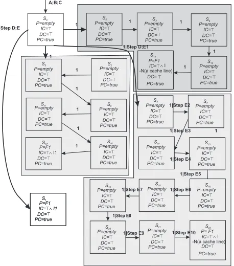
(1) cache hit and the cache is idle (execution trace A;B;C;D;E).

(2) cache miss and the cache is idle (execution trace A;B;C;D;E1;E2..E5).

(3) cache hit and the cache is busy (execution trace A;B;C;D;E1;E2..E6).

(4) cache miss and the cache is busy (execution trace A;B;C;D;E1;E2..E12).

On the graphs presented by the figure 4 and 5 we see that,

Figure 4: Symbolic execution steps of the executable timed model (ETM) for the assembly instruction

S0 P=empty

IC=>

DC=>

P C=true

S1 P=F1

IC=> ∧I1

DC=>

P C=true

S2 P=F1

IC=> ∧I1

DC=>

P C=true

S3 P=F1

IC=> ∧I1−

N(a cache line)

DC=>

P C=true

S4 P=F1

IC=> ∧I1−

N(a cache line)

DC=>

P C=true A;B;C

th(i)

tm trl+th(i)

[image:5.612.55.288.41.167.2]

trl+tm| STEP D;E

Figure 5: Symbolic execution steps of the time-accurate model (TAM) for the assembly instruction

concerning the scenario (1)–i.e., from the stateS0toS1, after

one clock cycle: (A) the pipeline fetches the instruction thus its state moves from(P=empty)to(P=F1), (B) the in-struction cache contains the inin-struction so its state moves from (IC=>)to(IC=>∧I1), (C) the cache state(DC)as well as theP Cstay at the same state. Now, in order to understand the interest behind abstracting the executable timed model, we focus on the last instruction of the model (instruction E). This instruction allows to know the time needed to get the instruc-tion from the instrucinstruc-tion cache. So in the presence of a cache miss (or pipeline stalls) if we choose to build the tree using an executable timed model (The simplest implementation which use the clock as the base cycle) it may lead to unnecessary in-termediate states since the processor is waiting during the time returned by the instruction E. A more efficient implementation is the time-accurate model. It is achieved when returning the next processor state that is different from the current one as well as the number of clock cycles required to reach this pro-cessor state. Like we see on the figure 5 , this abstraction does not introduce any loss of precision. Thus we explore the same

[image:5.612.309.530.333.424.2]

paths .i.e. the scenarios presented above. But now instead of executing the program clock cycle by clock cycle, we compute immediately the set of pertinent “intermediate states”. So the previous scenarios become:

(1) cache hit and the cache is idle takesthclock cycles. (2) cache miss and the cache is idle takestmclock cycles. (3) cache hit and the cache is busy. takesth+trlclock cycles. (4) cache miss and the cache is busy takestm+trlclock cy-cles.

Now if we compare the graph on figure 5 with the one pre-sented on figure 4 we conclude easily that:

- The number of the generated states has decreased (the ex-ecution trace has decreased from A;B;C;D;E0;E1;E2..En to A;B;C;D;E).

- Both of them contain the same information (we do not intro-duce any loss of precision).

6

Merging states

The symbolic execution allows to represent all the states that the processor may reach at each program point. So, the num-ber of the generated states during the execution increases ex-ponentially. Assuming thatρrepresents the pipeline depth,σ

denotes the maximal efficiency of the processor i.e. the num-ber of instructions that are handled per clock-cycle, andη de-notes the number of instructions of the code snippet, then an upper bound of the number of the states generated is:3σ η ρ

To avoid this exponential states explosion, the second part of the analysis consists in merging those states relying on the loss of precision we are ready to accept. Indeed, we developed a merging policy (see [15] for details) to reduce the previous exponential increase to a linear one which is equal to:

γ σ η3ρ+λ_{whereγis the maximum number of set of}

“inter-mediate states”.

7

Conclusion and future work

We presented a part of our analysis method to compute an up-per estimation of the WCET that can be parameterized by cur-rent complex hardware architecture, the only requirement is that an executable time-accurate model of the target system is available.

Instead of trying to build semi-automatically from the for-mal hardware description of the target system the black boxes of the analyzer that abstract the behavior of the target sys-tem [13], we have described a new approach that: Uses a sim-ple model–.i.e, it is easy to develop this model or to modify it (1). Can easily adapted to complex hardware architectures (2). Takes into account all the dependencies and the inter-actions that happen between the processor’s units during the execution (3).

This approach is currently being implemented and fully tested with time-accurate model of PPC 603e [3, 4] as well as multi-core PPC 5554 processors.

References

[1] J. C. King.,“Symbolic Execution and Program Testing,”, Communications of the ACM, V19, 7/76.

[2] J. A. Darringer., “The application of program verification techniques to hardware verification”, Annual ACM IEEE Design Automation Conference pp. 376–381, 88 [3] MOTOROLA., MPC603e EC603e RISC

Microproces-sors User’s Manual with Supplement for PowerPC 603TM_{Microprocessor, 97}

[4] Freescale Semiconductor., PowerPC 603 RISC Micro-processors Technical Summary, 94

[5] C. Ferdinand and D. Kastner and M. Langenbach and F. Martin and M. Schmidt and J. Schneider and H. Theil-ing and S. ThesTheil-ing and R. Wilhelm., “Run-Time Guar-antees for Real-Time Systems – The USES Approach”, GI Jahrestagung, pp. 410–419, 99

[6] J. Souyris, E. Le Pavec, G. Himbert, V. Jégu, G. Borios and R. Heckmann., “Computing the worst case execution time of an avionics program by abstract interpretation”

[7] P. Lokuciejewski, H. Falk, M. Schwarzer, P. Mar-wedel, H. Theiling., “Influence of procedure cloning on WCET prediction” Proceedings of the 5th IEEE/ACM international conference on Hardware/software code-sign Salzburg, Austria, pp. 137–142, 07

[8] R. Heckmann, C. Ferdinand., “Worst case execution time prediction by static program analysis” 18th Parallel and Distributed Processing Symposium, pp. 125–134, 04/04 [9] P. Cousot., “Semantic Foundations of Program

Analy-sis”, Program Flow Analysis: Theory and Applications, New Jersey pp. 303–342, 81

[10] P. Cousot and R. Cousot., “Abstract interpretation: a uni-fied lattice model for static analysis of programs by con-struction or approximation of fixpoints”, Fourth Annual ACM SIGPLAN-SIGACT Symposium on Principles of Programming Languages, Los Angeles, California, pp. 238–252, 77

[11] Y. Zhang., “Evaluation of Methods for Dynamic Time Analysis for CC-Systems AB” Technical Report Mälardalen University, 08/05

[12] D. B. Stewart., “Measuring Execution Time and Real-Time Performance” Embedded Systems Conference, San Francisco, 04/01

[13] M. Schlickling and M. Pister., “A Framework for Static Analysis of VHDL Code” 7th Intl. Workshop on WCET Analysis, 07

[14] S.Thesing., Safe and Precise WCET Determination by Abstract Interpretation of Pipeline Models, 04

[15] B. Benhamamouch and B. Monsuez and F. Védrine., “Computing WCET using symbolic execution”, 2nd In-ternational Workshop on Verification and Evaluation of Computer and Communication Systems. Leeds GB , 08/08