Sparse Communication for Distributed Gradient Descent
Alham Fikri Aji and Kenneth Heafield School of Informatics, University of Edinburgh
10 Crichton Street Edinburgh EH8 9AB Scotland, European Union
[email protected],[email protected]
Abstract
We make distributed stochastic gradient descent faster by exchanging sparse up-dates instead of dense upup-dates. Gradi-ent updates are positively skewed as most updates are near zero, so we map the 99% smallest updates (by absolute value) to zero then exchange sparse matrices. This method can be combined with quan-tization to further improve the compres-sion. We explore different configura-tions and apply them to neural machine translation and MNIST image classifica-tion tasks. Most configuraclassifica-tions work on MNIST, whereas different configurations reduce convergence rate on the more com-plex translation task. Our experiments show that we can achieve up to 49% speed up on MNIST and 22% on NMT without damaging the final accuracy or BLEU.
1 Introduction
Distributed computing is essential to train large neural networks on large data sets (Raina et al.,
2009). We focus on data parallelism: nodes jointly optimize the same model on different parts of the training data, exchanging gradients and param-eters over the network. This network commu-nication is costly, so prior work developed two ways to approximately compress network traffic: 1-bit quantization (Seide et al.,2014) and sending sparse matrices by dropping small updates (Strom,
2015;Dryden et al.,2016). These methods were developed and tested on speech recognition and toy MNIST systems. In porting these approxima-tions to neural machine translation (NMT) (˜Neco
and Forcada,1996;Bahdanau et al.,2014), we find that translation is less tolerant to quantization.
Throughout this paper, we compare neural ma-chine translation behavior with a toy MNIST sys-tem, chosen because prior work used a similar system (Dryden et al., 2016). NMT parameters are dominated by three large embedding matrices: source language input, target language input, and target language output. These matrices deal with vocabulary words, only a small fraction of which are seen in a mini-batch, so we expect skewed gra-dients. In contrast, MNIST systems exercise ev-ery parameter in evev-ery mini-batch. Additionally, NMT systems consist of multiple parameters with different scales and sizes, compared to MNIST’s 3-layers network with uniform size. More for-mally, gradient updates have positive skewness co-efficient (Zwillinger and Kokoska, 1999): most are close to zero but a few are large.
2 Related Work
An orthogonal line of work optimizes the SGD algorithm and communication pattern. Zinke-vich et al. (2010) proposed an asynchronous ar-chitecture where each node can push and pull the model independently to avoid waiting for the slower node. Chilimbi et al. (2014) and Recht et al. (2011) suggest updating the model without a lock, allowing race conditions. Additionally,
Dean et al. (2012) run multiple minibatches be-fore exchanging updates, reducing the communi-cation cost. Our work is a more continuous ver-sion, in which the most important updates are sent between minibatches. Zhang et al.(2015) down-weight gradients based on stale parameters.
Approximate gradient compression is not a new idea. 1-Bit SGD (Seide et al., 2014), and later Quantization SGD (Alistarh et al., 2016), work by converting the gradient update into a 1-bit ma-trix, thus reducing data communication signifi-cantly.Strom(2015) proposed threshold
tion, which only sends gradient updates that larger than a predefined constant threshold. However, the optimal threshold is not easy to choose and, more-over, it can change over time during optimization.
Dryden et al.(2016) set the threshold so as to keep a constant number of gradients each iteration.
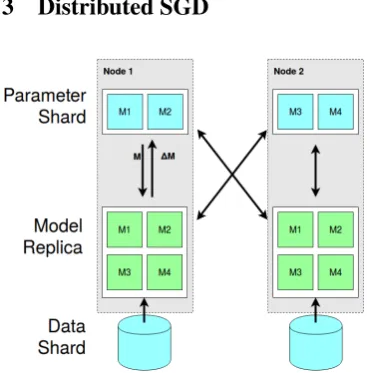
[image:2.595.71.255.161.348.2]3 Distributed SGD
Figure 1: Distributed SGD architecture with pa-rameter sharding.
We used distributed SGD with parameter shard-ing (Dean et al.,2012), shown in Figure1. Each of theNworkers is both a client and a server. Servers are responsible for1/Nth of the parameters.
Clients have a copy of all parameters, which they use to compute gradients. These gradients are split into N pieces and pushed to the appro-priate servers. Similarly, each client pulls param-eters from all servers. Each node converses with all N nodes regarding1/Nth of the parameters, so bandwidth per node is constant.
4 Sparse Gradient Exchange
We sparsify gradient updates by removing the R% smallest gradients by absolute value, dubbing this Gradient Dropping. This approach is slightly dif-ferent fromDryden et al.(2016) as we used a sin-gle threshold based on absolute value, instead of dropping the positive and negative gradients sepa-rately. This is simpler to execute and works just as well.
Small gradients can accumulate over time and we find that zeroing them damages convergence. FollowingSeide et al.(2014), we remember resid-uals (in our case dropped values) locally and add them to the next gradient, before dropping again.
Algorithm 1 Gradient dropping algorithm given gradient∇and dropping rateR.
functionGRADDROP(∇,R)
∇+ =residuals
Selectthreshold: R% of|∇|is smaller dropped←0
dropped[i]← ∇[i]∀i:|∇[i]|> threshold residuals← ∇ −dropped
returnsparse(dropped)
end function
Gradient Dropping is shown in Algorithm 1. This function is applied to all data transmissions, including parameter pulls encoded as deltas from the last version pulled by the client. To compute these deltas, we store the last pulled copy server-side. Synchronous SGD has one copy. Asyn-chronous SGD has a copy per client, but the server is responsible for1/Nth of the parameters forN clients so memory is constant.
Selection to obtain the threshold is expensive (Alabi et al.,2012). However, this can be approxi-mated. We sample0.1%of the gradient and obtain the threshold by running selection on the samples. Parameters and their gradients may not be on comparable scales across different parts of the neural network. We can select a threshold locally to each matrix of parameters or globally for all pa-rameters. In the experiments, we find that layer normalization (Lei Ba et al.,2016) makes a global threshold work, so by default we use layer normal-ization with one global threshold. Without layer normalization, a global threshold degrades conver-gence for NMT. Prior work used global thresholds and sometimes column-wise quantization.
5 Experiment
We experiment with an image classification task based on MNIST dataset (LeCun et al., 1998) and Romanian→English neural machine transla-tion system.
For our image classification experiment, we build a fully connected neural network with three 4069-neuron hidden layers. We use AdaGrad with an initial learning rate of 0.005. The mini-batch size of 40 is used. This setup is identical to Dry-den et al.(2016).
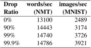
Drop words/sec images/sec
Ratio (NMT) (MNIST)
0% 13100 2489
90% 14443 3174
99% 14740 3726
[image:3.595.100.260.62.146.2]99.9% 14786 3921
Table 1: Training speed with various drop ratios.
119M parameters. The default batch size is 80. We save and validate every 10000 steps. We pick 4 saved models with the highest validation BLEU and average them into the final model. AmuNMT (Junczys-Dowmunt et al.,2016) is used for decoding with a beam size of 12. Our test system has PCI Express 3.0 x16 for each of 4 NVIDIA Pascal Titan Xs. All experiments used asynchronous SGD, though our method applies to synchronous SGD as well.
5.1 Drop Ratio
To find an appropriate dropping ratio R%, we tried 90%, 99%, and 99.9% then measured perfor-mance in terms of loss and classification accuracy or translation quality approximated by BLEU ( Pa-pineni et al., 2002) for image classification and NMT task respectively.
Figure 3 shows that the model still learns af-ter dropping 99.9% of the gradients, albeit with a worse BLEU score. However, dropping 99% of the gradient has little impact on convergence or BLEU, despite exchanging 50x less data with offset-value encoding. Thex-axis in both plots is batches, showing that we are not relying on speed improvement to compensate for convergence.
Dryden et al.(2016) used a fixed dropping ratio of 98.4% without testing other options. Switching to 99% corresponds to more than a 1.5x reduction in network bandwidth.
For MNIST, gradient dropping oddly improves accuracy in early batches. The same is not seen for NMT, so we caution against interpreting slight gains on MNIST as regularization.
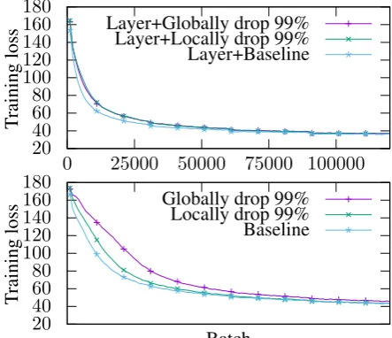
5.2 Local vs Global Threshold
Parameters may not be on a comparable scale so, as discussed in Section4, we experiment with lo-cal thresholds for each matrix or a global threshold for all gradients. We also investigate the effect of layer normalization. We use a drop ratio of 99% as suggested previously. Based on the results and
0 0.3 0.6
3000 6000 9000
Training
loss
99.9% drop rate 99% drop rate 90% drop rate baseline
0.94 0.96 0.98 1
accurac
y
[image:3.595.309.534.69.265.2]Batch
Figure 2: MNIST: Training loss and accuracy for different dropping ratios.
20 40 60 80 100 120 140 160 180
0 25000 50000 75000 100000
Training
loss
99.9% drop rate 99% drop rate 90% drop rate baseline
5 10 15 20 25 30 35
validation
BLEU
Batch
Figure 3: NMT: Training loss and validation BLEU for different dropping ratios.
due to the complicated interaction with sharding, we did not implement locally thresholded pulling, so only locally thresholded pushing is shown.
[image:3.595.310.531.346.542.2]0 0.3 0.6
3000 6000 9000
Training
loss
Layer+Globally drop 99% Layer+Locally drop 99% Layer+Baseline
0 0.3 0.6
Training
loss
Batch Globally drop 99%
[image:4.595.75.295.69.267.2]Locally drop 99% Baseline
Figure 4: MNIST: Comparison of local and global thresholds with and without layer normalization.
20 40 60 80 100 120 140 160 180
0 25000 50000 75000 100000
Training
loss
Layer+Globally drop 99% Layer+Locally drop 99% Layer+Baseline
20 40 60 80 100 120 140 160 180
Training
loss
Batch Globally drop 99%
Locally drop 99% Baseline
Figure 5: NMT: Comparison of local and global thresholds with and without layer normalization.
5.3 Convergence Rate
While dropping gradients greatly reduces the com-munication cost, it is shown in Table1that overall speed improvement is not significant for our NMT experiment. For our NMT experiment with 4 Ti-tan Xs, communication time is only around 13% of the total training time. Dropping 99% of the gradient leads to 11% speed improvement. Addi-tionally, we added an extra experiment of NMT with batch-size of 32 to give more communication cost ratio. In this scenario, communication is 17%
of the total training time and we see a 22% aver-age speed improvement. For MNIST, communi-cation is 41% of the total training time and we see a 49% average speed improvement. Computation got faster by reducing multitasking.
We investigate the convergence rate: the combi-nation of loss and speed. For MNIST, we train the model for 20 epochs as mentioned inDryden et al.
(2016). For NMT, we tested this with batch sizes of 80 and 32 and trained for 13.5 hours.
0.94 0.96 0.98 1
0 100 200 300 400 500
Accurac
y
time (second) 99% drop rate
baseline
Figure 6: MNIST classification accuracy over time.
As shown in Figure 6, our baseline MNIST experiment reached 99.28% final accuracy, and reached 99.42% final accuracy with a 99% drop rate. It also shown that it has better convergence rate in general with gradient dropping.
20 40 60 80 100 120
0 3 6 9 12
Validation
loss 99% drop rate (b80)99% drop rate (b32)baseline (b80) baseline (b32)
5 10 15 20 25 30 35
validation
BLEU
[image:4.595.310.529.214.324.2]Hours
Figure 7: NMT validation BLEU and loss over time.
Our NMT experiment result is shown in Table
[image:4.595.73.295.340.531.2] [image:4.595.310.531.474.671.2]Experiment Final Time to reach
%BLEU 33% BLEU
batch-size 80
+ baseline 34.51 2.6 hours + 99% grad-drop 34.40 2.7 hours batch-size 32
[image:5.595.74.285.62.173.2]+ baseline 34.16 4.2 hours + 99% grad-drop 34.08 3.2 hours
Table 2: Summary of BLEU score obtained.
Our algorithm converges 23% faster than the base-line when the batch size is 32, and nearly the same with a batch size of 80. This in a setting with fast communication: 15.75 GB/s theoretical over PCI express 3.0 x16.
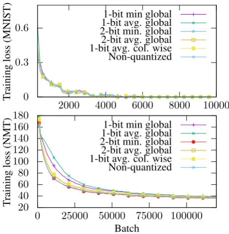
5.4 1-Bit Quantization
We can obtain further compression by applying 1-bit quantization after gradient dropping. Strom
(2015) quantized simply by mapping all surviving values to the dropping threshold, effectively the minimum surviving absolute value. Dryden et al.
(2016) took the averages of values being quan-tized, as is more standard. They also quantized at the column level, rather than choosing centers globally. We tested 1-bit quantization with 3 dif-ferent configurations: threshold, column-wise av-erage, and global average. The quantization is ap-plied after gradient dropping with a 99% drop rate, layer normalization, and a global threshold.
Figure 8 shows that 1-bit quantization slows down the convergence rate for NMT. This differs from prior work (Seide et al.,2014;Dryden et al.,
2016) which reported no impact from 1-bit quan-tization. Yet, we agree with their experiments: all tested types of quantization work on MNIST. This emphasizes the need for task variety in ex-periments.
NMT has more skew in its top 1% gradients, so it makes sense that 1-bit quantization causes more loss. 2-bit quantization is sufficient.
6 Conclusion and Future Work
Gradient updates are positively skewed: most are close to zero. This can be exploited by keeping 99% of gradient updates locally, reducing com-munication size to 50x smaller with a coordinate-value encoding.
Prior work suggested that 1-bit quantization can be applied to further compress the communication.
0 0.3 0.6
2000 4000 6000 8000 10000
Training
loss
(MNIST)
1-bit min global 1-bit avg. global 2-bit min. global 2-bit avg. global 1-bit avg. col. wise Non-quantized
20 40 60 80 100 120 140 160 180
0 25000 50000 75000 100000
Training
loss
(NMT)
[image:5.595.308.542.68.308.2]Batch 1-bit min global 1-bit avg. global 2-bit min. global 2-bit avg. global 1-bit avg. col. wise Non-quantized
Figure 8: Training loss for different quantization methods.
However, we found out that this is not true for NMT. We attribute this to skew in the embedding layers. However, 2-bit quantization is likely to be sufficient, separating large movers from small changes. Additionally, our NMT system consists of many parameters with different scales, thus layer normalization or using local threshold per-parameter is necessary. On the hand side, MNIST seems to work with any configurations we tried.
Our experiment with 4 Titan Xs shows that on average only 17% of the time is spent communi-cating (with batch size 32) and we achieve 22% speed up. Our future work is to test this approach on systems with expensive communication cost, such as multi-node environments.
Acknowledgments
In-stitute under the EPSRC grant EP/N510129/1.
References
Tolu Alabi, Jeffrey D Blanchard, Bradley Gordon, and Russel Steinbach. 2012. Fast k-selection algorithms for graphics processing units. Journal of Experi-mental Algorithmics (JEA)17:4–2.
Dan Alistarh, Jerry Li, Ryota Tomioka, and Milan Vojnovic. 2016. QSGD: randomized quan-tization for communication-optimal stochas-tic gradient descent. CoRR abs/1610.02132.
http://arxiv.org/abs/1610.02132.
Dzmitry Bahdanau, Kyunghyun Cho, and Yoshua Bengio. 2014. Neural machine translation by jointly learning to align and translate. CoRR abs/1409.0473. http://arxiv.org/abs/1409.0473. Trishul M Chilimbi, Yutaka Suzue, Johnson Apacible,
and Karthik Kalyanaraman. 2014. Project adam: Building an efficient and scalable deep learning training system. In OSDI. volume 14, pages 571– 582.
Jeffrey Dean, Greg Corrado, Rajat Monga, Kai Chen, Matthieu Devin, Mark Mao, Andrew Senior, Paul Tucker, Ke Yang, Quoc V Le, et al. 2012. Large scale distributed deep networks. In Advances in neural information processing systems. pages 1223– 1231.
Nikoli Dryden, Sam Ade Jacobs, Tim Moon, and Brian Van Essen. 2016. Communication quantization for data-parallel training of deep neural networks. In Proceedings of the Workshop on Machine Learn-ing in High Performance ComputLearn-ing Environments. IEEE Press, pages 1–8.
Marcin Junczys-Dowmunt, Tomasz Dwojak, and Hieu Hoang. 2016. Is neural machine translation ready for deployment? A case study on 30 translation directions. In Program of the 13th International Workshop on Spoken Language Translation (IWSLT 2016).
Yann LeCun, L´eon Bottou, Yoshua Bengio, and Patrick Haffner. 1998. Gradient-based learning applied to document recognition. Proceedings of the IEEE 86(11):2278–2324.
J. Lei Ba, J. R. Kiros, and G. E. Hinton. 2016. Layer Normalization. ArXiv e-prints.
Ram´on P ˜Neco and Mikel L Forcada. 1996. Beyond mealy machines: Learning translators with recurrent neural networks. InProceedings of the 1996 Inter-national Neural Network Society Annual Meeting. San Diego, California, USA.
Kishore Papineni, Salim Roukos, Todd Ward, and Wei-Jing Zhu. 2002. BLEU: A method for automatic evalution of machine translation. In Proceedings
40th Annual Meeting of the Association for Com-putational Linguistics. Philadelphia, PA, pages 311– 318.
Rajat Raina, Anand Madhavan, and Andrew Y Ng. 2009. Large-scale deep unsupervised learning using graphics processors. InProceedings of the 26th an-nual international conference on machine learning. ACM, pages 873–880.
Benjamin Recht, Christopher Re, Stephen Wright, and Feng Niu. 2011. Hogwild: A lock-free approach to parallelizing stochastic gradient de-scent. In J. Shawe-Taylor, R. S. Zemel, P. L. Bartlett, F. Pereira, and K. Q. Weinberger, editors, Advances in Neural Information Processing Sys-tems 24, Curran Associates, Inc., pages 693–701.
http://papers.nips.cc/paper/4390-hogwild-a-lock- free-approach-to-parallelizing-stochastic-gradient-descent.pdf.
Frank Seide, Hao Fu, Jasha Droppo, Gang Li, and Dong Yu. 2014. 1-bit stochastic gradi-ent descgradi-ent and application to data-parallel
distributed training of speech DNNs. In
Interspeech. https://www.microsoft.com/en- us/research/publication/1-bit-stochastic-gradient- descent-and-application-to-data-parallel-distributed-training-of-speech-dnns/.
Rico Sennrich, Barry Haddow, and Alexandra Birch. 2016. Edinburgh neural machine translation sys-tems for WMT 16. InProceedings of the ACL 2016 First Conference on Machine Translation (WMT16). Nikko Strom. 2015. Scalable distributed dnn training using commodity gpu cloud computing. In INTER-SPEECH. volume 7, page 10.
Wei Zhang, Suyog Gupta, Xiangru Lian, and Ji Liu. 2015. Staleness-aware async-sgd for dis-tributed deep learning. CoRR abs/1511.05950.
http://arxiv.org/abs/1511.05950.
Martin Zinkevich, Markus Weimer, Lihong Li, and Alex J Smola. 2010. Parallelized stochastic gradient descent. InAdvances in neural information process-ing systems. pages 2595–2603.