Forecasting Daily Stock Volatility Using GARCH CJ Type Models with Continuous and Jump Variation

(1)

Munich Personal RePEc Archive

Forecasting Daily Stock Volatility Using

GARCH-CJ Type Models with

Continuous and Jump Variation

BOUSALAM, Issam and HAMZAOUI, Moustapha and

ZOUHAYR, Otman

Abdelmalek Essaädi University of Tangier - Morocco,

Albanki-Alternative Banking Institute - France

20 January 2016

(2)

Forecasting Daily Stock Volatility Using GARCH-CJ

Type Models with Continuous and Jump Variation

Issam BOUSALAM∗a

, Moustapha HAMZAOUIb, and Otman ZOUHAYRc

a,b_{Department of Economics, Abdelmalek Essaädi University of Tangier - Morocco}

c_{Albanki-Alternative Banking Institute - France}

January 20, 2016

Abstract

In this paper we decompose the realized volatility of the GARCH-RV model into continuous sample path variation and discontinuous jump variation to provide a practical and robust framework for non-parametrically measuring the jump component in asset return volatility. By using 5-minute high-frequency data of MASI Index in Morocco for the period (January 15, 2010 - January 29, 2016), we estimate parameters of the constructed GARCH and EGARCH-type models (namely, GARCH, GARCH-RV, GARCH-CJ, EGARCH, EGARCH-RV, and EGARCH-CJ) and evaluate their predictive power to forecast future volatility. The results show that the realized volatility and the continuous sample path variation have certain predictive power for future volatility while the discontinuous jump variation contains relatively less information for forecasting volatility. More interestingly, the findings show that the GARCH-CJ-type models have stronger predictive power for future volatility than the other two types of models. These results have a major contribution in financial practices such as financial derivatives pricing, capital asset pricing, and risk measures.

JEL-Classification:C22, F37, F47, G17.

Keywords: GARCH-CJ, Jumps variation, Realized volatility, MASI Index, Morocco.

(3)

1 Introduction

A common finding in much of the empirical finance literature is that asset returns volatility exhibits "clustering" and "persistence" features. This is why Engle (1982) proposed the AutoRegressive Conditional heteroskedasticity (ARCH) model which was generalized later by Bollerslev (1986) to take into account bigger regression order and proposed the GARCH model. Nelson (1991) found that the asset volatility is "asymmetric" relatively to bad and good news on the market, then he modified the GARCH model and built an exponential GARCH model (EGARCH). These models (GARCH and EGARCH) were found to be more powerful in predicting future volatility (Andersen and Bollerslev, 1998).

Despite the fact that GARCH style models have been continuously proved to be stronger for predicting asset returns volatility, seeking to improve the accuracy of future volatility prediction is an endless process and constitutes the premise of quantitative financial analysis. This is because measuring and predicting accurately the asset returns volatility has too much practical uses in financial asset pricing, financial derivative pricing, and financial risk management.

In order to enhance the accuracy of volatility forecasting, Koopman et al. (2005) introduced the realized volatility (RV) as an exogenous variable into the volatility equation of GARCH model. They built a GARCH-RV model and found that the it has stronger predictive power than the traditional GARCH model. The same results were found by Fuertes et al. (2009) and Frijns et al. (2011).

But in realistic financial markets, the process of asset volatility is not completely continuous but contains some jump components. In fact, Andersen et al. (2007) and Huang et al. (2013) studied the HAR-type RV model and found that model built with continuous sample path variation and discontinuous jump variation that decomposed from RV has stronger power than the undecomposed HAR-RV model in measuring and predicting the asset volatility.

Based on these findings, we estimate that it makes sense to split the exogenous variable RV introduced in GARCH-RV model into a continuous sample path variation and discontinuous jumps variation in order to further enhance the predictive power of GARCH-RV model. Similarly, in this paper we will also extend the EGARCH model to an EGARCH-RV model and an EGARCH-CJ model. Next, we estimate parameters of the above mentioned models and evaluate their forecasting power for the future volatility to identify which volatility model has stronger power for the asset volatility measurement and prediction. This by using the 5-minute high-frequency data of the broad based Moroccan All Shares Index for a 5 years period ranging from January 15, 2010 to January 29, 2016.

(4)

2 Model Specification

2.1 GARCH-CJ Model building

2.1.1 GARCH-RV Model Construction

Stock return volatility cannot be directly observable but can be measured in the asset return series. Financial literature shows that return volatility is "clustering" and "persistent" over time. Engle (1982) proposed the AutoRegressive Conditional heteroskedasticity (ARCH) model that captures the clustering feature and Bollerslev (1986) generalized it to take into account bigger regression order and proposed the GARCH model. Scholars generally use the GARCH(1,1) model described by:

rt= ln

_I

t

It−1

=E(rt|Ψt−1) +ǫt

ǫt=σt·zt , zt∼ψ(0,1, v) (1)

σ_t2=ω+αǫ2_t−1+βσ 2

t−1

Itis the price of the index at timetand Ψt−1 contains all information up to dayt−1. ǫt are the

random innovations (surprises) withE(ǫt) = 0 and they are split into a white noise disturbanceztand

a time-dependent standard deviationσtcharacterizing the typical size of the error terms. ψ(.) marks

a conditional density function andv denotes a vector of parameters needed to specify the probability distribution of zt. σt is the volatility andω,α andβ are parameters to be estimated.

Seeking to improve the explanatory and the predictive power of the traditional GARCH model, Koopman et al. (2005) incorporated the Realized Volatility (RV) as an exogenous variable into the volatility model GARCH(1,1) and built the GARCH-RV model expressed as follows:

rt=E(rt|Ψt−1) +ǫt , ǫt=σt·zt

σ2_t =ω+αǫ2_t−₁+βσ 2

t−₁+λRVt−1 (2)

λis a parameter to be estimated as forω,α and β, and RVt−1 is the realized volatility at time

t₋1. Martens (2002) and Koopman et al. (2005) emphasized the importance of using high-frequency intraday returns to the measuring and forecasting of volatility and expressed the realized volatility as a function of overnight return variance.

RVt= N

X

i=1

r2_t,i+r_t,n2 =

M

X

j=1

r2_t,j , M =N + 1 (3)

By assuming N equally divided parts of a trading day, rt,1 represents the log-return for the first period (part) of the day where rt,1 = ln(It,1/It,0) and It,0 is the opening price at Day t, rt,2 is the log-return for the second period; ..., and rt,N expresses the Nth return at Day t. Finally,

(5)

2.1.2 GARCH-CJ Model Construction

There is empirical evidence that stock markets exhibit fractal features and financial asset price volatility is not continuous but rather generated by a jump process. The nonlinear properties of the stock market volatility is almost due to big information shocks and investors’ irrational behaviors. Therein, in order to improve the predictive power of the GARCH-RV model, Andersen et al. (2007) decomposed the realized volatility (RV) in model (2) into a continuous sample path variation denoted Cj and a discontinuous jump variationJt.

Alternatively, Barndorff-Nielsen and Shephard (2006) introduced the Realized Bipower Variation (RBV) with more robustness properties described by:

RBV_t[r,s]=

( _h

M

1−(r+s)/2)M−1

X

j=1

rj,t

rrj+1,t

s, r, s_≥0. (4)

Where r and s are constants1, h is a fix time interval and M is the sample frequency within intervalh. Barndorff-Nielsen and Shephard (2006) demonstrated that when a stochastic volatility and an infrequent jumps process exist, then the difference between RV and RBV estimates the quadratic variation of the jump componentJtwhen M → ∞.

RVt−RBVt M

→∞

−−−−→Jt. (5)

Given a limited sample size, the jumps variationJtcalculated in (5) may not be always positive and to overcome this issue, we treatJt in the following way:

Jt= Max[RVt−RBVt,0]. (6)

When calculating the discontinuous jumps variation Jt a problem of accuracy occurs for an

intraday data sampled at unequal frequency. This is why Barndorff-Nielsen and Shephard (2006) introduced a Ztstatistic to test for Jt. Zt is described by:

Zt=

(RVt−RBVt)RV

−₁

t

q

Max(1, RT Qt/RBVt2)(1/M) (π/2) +π−5

−→ N(0,1). (7)

Where

RT Qt=M µ−₄_/3₃

M M −4

_XM

j=4

rt,j−4

4/3rt,j−2

4/3rt,j4/3, (8)

µ₄_/₃ = E

|Zt|4/3

= 22/3Γ

₇ 6 Γ ₁ 2

−₁!

.

RT Qt is the Realized Tripower Quarticity which is an asymptotically unbiased estimator of

integrated quarticity in the absence of microstructure noise.

The calculation ofRBVt relies mainly on the sampling frequency of intraday data which might

result in some convergence issues when the sampling frequency is sufficiently high. This is due to

1_Usually_r₌_s_{= 1 is given so that}_RBV[1,1]

t =

PM−1

j=1 |rj,t|

r_|r

(6)

several factors and one of these is the market microstructure. Andersen et al. (2012) introduced the Median Realized Volatility (M edRVt) as a robust estimator for Jt instead of the biased RVt. The

alternative M edRVtuses two-sided truncation, picking the median of three adjacent absolute returns

and is expressed by (9). Similarly, RT Qt used for Zt calculation in (7) is replaced by M edRT Qt

described hereafter by (10).

M edRVt=

π 6−4√3 +π

_M

M₋2

×

M−1

X

i=2

M ed(_|rt,i−1|,|rt,i|,|rt,i+1|)2 (9)

M edRT Qt=

3πM 9π+ 72₋52√3

_M

M −2

×

M−1

X

i=2

M ed(_|rt,i−1|,|rt,i|,|rt,i+1|)4. (10)

By replacingRVtand RT Qt in (7) with M edRVt and M edRT Qt respectively, we calculate the

Zt statistic and get the estimator for both discontinuous jump variation Jt and continuous sample

path variation Cj at 1−α significance level. In this paper, based on previous research, we choose a

confidence levelα of 99%. Jt and Ct are then defined as:

Jt=I(Zt> φα)(RVt−M edRVt), (11)

Ct=I(Zt≤φα)RVt+I(Zt> φα)M edRVt. (12)

Finally, according to the aboveRVtdecomposition intoCtandJt, the GARCH-RV model in (2)

becomes the GARCH-CJ model expressed as follows:

σ2_t =ω+αǫ2_t−1+βσ 2

t−1+λCt−1+γJt−1 (13)

2.2 EGARCH-CJ Model specification

In response to the weakness of traditional GARCH model to capture all the leptokurtosis of the error terms and to handle the asymmetric responses of volatility, Nelson (1991) constructed the Exponential GARCH (EGARCH) model on the basis of the baseline GARCH model. Most commonly, researchers use the EGARCH(1,1) model described by:

lnσ2_t =ω+α |zt−1| −E[|zt−1|]

+βln(σ_t2−1) +θzt−1. (14)

Following the method discussed in Section 2.1.1, we get the EGARCH-RV model by introducing the log of the one-period-lagged realized volatility (RVt−1). Thus, equation (14) becomes:

lnσ_t2 =ω+α _|zt−1| −E[|zt−1|]

+βln(σ_t2−1) +θzt−1+λln(RVt−1). (15)

(7)

obtain the EGARCH-CJ model described as follows:

rt=E(rt|Ψt−₁) +ǫ_t , ǫ_t=σ_t·z_t

lnσ_t2=ω+α _|zt−1| −E[|zt−1|]

+βln(σ2_t−1) +θzt−1+λln(Ct−1) +γln(Jt−1+ 1). (16)

3 Empirical Results and Comparative Analysis of Models’

Predic-tive Power

3.1 Data and Empirical Properties

3.1.1 Sample Statistics

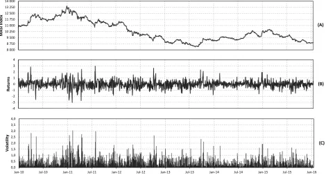
Our data set is the Moroccan All Shares Index (MASI), recorded at 5 minutes (5-min) intervals during the sample period of January 15, 2010 to January 29, 2016. Data is acquired from Bloombergr_.

The Casablanca Stock Exchange opens at 9:30 (GMT) and the first record of the MASI index for that day is registered at 9:31. The market closes at 15:30 (GMT) and the last record of the day is registered at 15:31. Therefore, considering a 5-min intervals during one trading day and by using the moving average interpolation for missed data we obtain 144 daily index records. Overall, our sample period consists of 1,506 days. We eliminated weekends and holidays during which the market was closed.

-4 -3 -2 -1 0 1 2 3 4 R e tur ns (B) 8 000 8 750 9 500 10 250 11 000 11 750 12 500 13 250 14 000 MA S I I nde x (A) 0,0 0,5 1,0 1,5 2,0 2,5 3,0 3,5 4,0

Jan-10 Jul-10 Jan-11 Jul-11 Jan-12 Jul-12 Jan-13 Jul-13 Jan-14 Jul-14 Jan-15 Jul-15 Jan-16

V o la tilit y (C)

[image:7.595.64.535.391.644.2]

(A) MASI Index level (B) 5-min returns (log difference, in percent) (C) 5-min volatility (absolute return, in percent). Sample period is January 15, 2010 - January 29, 2016 (216,864 5-mins, 1,506 days). Data source: Bloombergr

Figure 1: Moroccan All Shares Index (MASI) at 5-min intervals

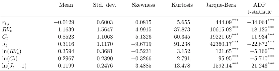
Table 1 below presents descriptive statistics of all variables needed to estimate the GARCH-type models described before, i.e. intraday returns rt,i, Realized Volatility RVt, continuous sample path

variationCtand discontinuous jump variationJt, and their respective logarithms: ln(RVt), ln(Ct) and

(8)

[image:8.595.59.539.81.203.2]

Table 1: Summary Statistics of Study’s Variables

Mean Std. dev. Skewness Kurtosis Jarque-Bera ADF t-statistic

rt,i −0.0129 0.6003 0.0815 5.655 444.09*** −34.064***

RVt 1.1639 1.5647 −4.9915 37.873 10615.02*** −18.125***

Ct 0.8523 1.1063 −5.1326 60.345 19221.69*** −11.934***

Jt 0.3116 1.1170 −9.6719 91.238 42360.17*** −22.872***

ln(RVt) 0.3594 0.3681 −0.5231 3.152 121.65*** −5.166***

ln(Ct) 0.2967 0.2390 −0.3266 2.791 95.95*** −5.710***

ln(Jt+ 1) 0.1199 0.2476 −3.4885 13.478 1592.14*** −21.246*** (***_{) denotes significance at 1% level of significance.}

We can clearly observe from Table 1 that returnsrt,i and realized volatilityRVtare not normally

distributed. These are fat-tailed which implies that volatility in Moroccan stock market is high. Furthermore, the ADF t-statistics are all significant at 99% level of confidence, we can easily reject the null hypothesis of unit root existence in the series. This allows us to use the variables for further models analysis and estimation of parameters.

3.1.2 Estimation of Models’ parameters and Comparison

The method of estimation adopted in this paper is maximum likelihood, and parameters of the six competing models (GARCH, GARCH-RV, GARCH-CJ, EGARCH, RV and EGARCH-CJ) were estimated under two assumptions for errors distribution, i.e. the normal distribution and Student-t distribution. Goodness of fit is compared using the log-likelihood, Akaike Information Criterion (AIC) and Schwarz Information Criterion (SIC).

[image:8.595.57.539.590.709.2]

From Table 2 below, by comparing log-likelihood and information criterion AIC and SIC, we can see that the EGARCH-type models (i.e. EGARCH, EGARCH-RV and EGARCH-CJ) outperform the GARCH-type models (i.e. GARCH, GARCH-RV and GARCH-CJ) in terms of goodness of fit of the data. This means that volatility on the stock market has an asymmetric response relatively to bad news and good news. Furthermore, both of GARCH-type models and EGARCH-type models fit better the data when residuals are assumed to be following a Student-t distribution.

Table 2: Log-likelihood, AIC and SIC for GARCH-type Models and EGARCH-type Models

Gaussian distribution Student-t distribution

LL AIC SIC LL AIC SIC d.f. GARCH(1,1) -1288.76 1.715 1.726 -1245.90 1.659 1.674 5.935***

GARCH-RV -1262.13 1.729 1.732 -1236.18 1.693 1.711 6.344***

GARCH-CJ -1238.56 1.753 1.754 -1225.44 1.745 1.737 7.119***

EGARCH(1,1) -1288.49 1.716 1.730 -1245.54 1.660 1.678 5.926***

EGARCH-RV -1259.28 1.732 1.733 -1223.66 1.695 1.701 6.845***

EGARCH-CJ -1254.75 1.754 1.762 1219.25 1.711 1.712 6.731*** Note — LL is the log-likelihood score. d.f. are degrees of freedom of t-distribution and are all significant at 1% level of significance (***_{). LL, AIC and SIC were calculated using 5-min returns of the MASI Index for the period covering January 15, 2010 to January}

29, 2016.

(9)

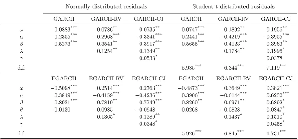
ln(RVt−1) are all significantly positive at 1% or 5% level of significance. This indicates that

volatil-ity in Moroccan stock market exhibits pronounced persistence and last period volatilvolatil-ity may affect current period volatility ; this result is consistent with (Koopman et al., 2005). As for the newly GARCH-CJ and EGARCH-CJ models, the coefficients (λ) for Ct are significantly positive at 10%

significance level, and the coefficients (γ) for Jt are non significant only when the residual errors in

the GARCH-CJ model are assumed to follow a Student-t distribution, otherwise significant.

[image:9.595.56.540.293.518.2]

These estimation results indicate that, in the Moroccan stock market, the lagged continuous sample path variation contains relatively more information for predicting the current volatility, while the lagged discontinuous jump variation contains relatively less information for forecasting. This finding leads us to test for which models has more predictive power for future volatility. Also, the leverage effect is negative (negative estimates for θ), meaning that the volatility in the stock market is more influenced by bad news than good news.

Table 3: Estimates of Parameters for GARCH-type Models and EGARCH-type Models

Normally distributed residuals Student-t distributed residuals

GARCH GARCH-RV GARCH-CJ GARCH GARCH-RV GARCH-CJ

ω 0.0883*** ₀_.₀₇₈₆** ₀_.₀₇₃₅** ₀_.₀₇₄₇*** ₀_.₁₈₉₂** ₀_.₁₉₅₆**

α 0.2355*** −0.2968*** −0.3341*** 0.2441*** −0.4219*** −0.3955***

β 0.5273*** ₀_.₃₅₄₁** ₀_.₃₉₁₇*** ₀_.₅₆₅₅*** ₀_.₄₁₂₃*** ₀_.₃₉₆₃**

λ 0.1254** ₀_.₁₃₄₉** ₀_.₁₇₈₄** ₀_.₁₉₉₆*

γ 0.0533* 0.0378

d.f. 5.935*** ₆_.₃₄₄*** ₇_.₁₁₉***

EGARCH EGARCH-RV EGARCH-CJ EGARCH EGARCH-RV EGARCH-CJ

ω −0.5098*** 0.2514*** 0.2763*** −0.4873*** 0.3649*** 0.3821***

α 0.3849*** ₋₀_.₄₁₅₉*** ₋₀_.₄₂₃₆*** ₀_.₃₉₀₆*** ₋₀_.₆₁₄₄*** ₀_.₆₂₃₂***

β 0.8031*** ₀_.₇₈₁₀** ₀_.₇₇₄₉*** ₀_.₈₂₆₀** ₀_.₆₉₇₁** ₀_.₆₈₉₂*

θ −0.0130 −0.0985 −0.0948 −0.0268 −0.0828 −0.0847*

λ 0.1365* ₀_.₁₂₈₉** ₀_.₁₄₃₇* ₀_.₁₅₁₀*

γ 0.0348* ₀_.₀₄₅₈*

d.f. 5.926*** 6.845*** 6.731***

Note — d.f. are degrees of freedom of t-distribution and are all significant at 1% level of significance. Models’ parameters are estimated using 5-min returns of the MASI Index for the period covering January 15, 2010 to January 29, 2016. ***_,**_{, and} *

denote significance at the 1%, 5%, and 10% significance level respectively.

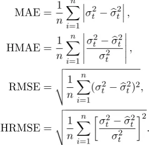
3.2 Forecasting Methodology and Evaluation Criteria

3.2.1 In-Sample Forecasting

(10)

MAE = 1 n n X i=1

σ2_t ₋σb2_t,

HMAE = 1

n n X i=1

σ_t2−σb_t2

σ2 t , RMSE = v u u t1 n n X i=1 (σ2

t −σbt2)2,

HRMSE = v u u t1 n n X i=1 _σ2

t −σbt2

σ2_t

2

.

(17)

Wheren denotes the size of the predictive sample, σ2_t is the real volatility substituted by RVt,

and σb2

t is the predicted volatility.

[image:10.595.224.372.70.213.2]

Values of in-sample predictive power indexes for the GARCH-type models and EGARCH-type models are listed in Table 4 below.

Table 4: In-Sample Forecast Evaluation

Errors following normal distribution Errors following t distribution MAE HMAE RMSE HRMSE MAE HMAE RMSE HRMSE GARCH(1,1) 3.5981 0.9837 7.1927 1.3671 3.5647 0.9846 7.2239 1.5410 GARCH-RV 3.5467 0.9216 6.8913 0.9180 3.4988 0.9517 7.2603 1.6131 GARCH-CJ 3.2830 0.8217 6.9516 0.8692 3.4207 0.8946 7.2554 1.6128 EGARCH(1,1) 3.5218 0.9610 7.0220 1.2593 3.5158 0.9126 6.9373 1.5416 EGARCH-RV 3.4894 0.9154 6.8556 1.1346 3.4791 0.8978 6.6210 1.1246 EGARCH-CJ 3.4412 0.8999 6.8373 1.1299 3.4697 0.8615 6.5431 1.1222

Our full sample consists of 216,864 observations (5-min returns) corresponding to 1,506 days from January 15, 2010 to January 29, 2016. GARCH and EGARCH-type models are estimated over the first 195,264 observations of the full sample, i.e. over the period January 15, 2010 to June 15, 2015

Table 4 shows that all values for CJ-type models are smaller than that of both GARCH-RV and GARCH type models consecutively. This leads us to conclude that in in-sample volatility forecasting, the GARCH-CJ-type models perform better than their counterparts and have more pre-dictive power. However, when comparing forecasting power of volatility models given normal and student-t distribution for residuals, the findings are mixed and inconclusive regarding which error dis-tribution assumption contributes better to boost the predictive power of the models. See that for the same given model of the six competing models, the four measures when assuming normal distribution for errors are not all smaller (alternatively, higher) than those for a student-t assumption for errors distribution, and judging the predictive power of models relies on which measure is used to for the comparison.

3.2.2 Out-Of-Sample Forecasting

[image:10.595.58.539.328.444.2]

(11)

from January 15, 2010 to June 15, 2015, and the second part used for prediction covers the remaining 150 days till January 29, 2016. We still use the same loss function to evaluate the predictive power as for in-sample forecasting.

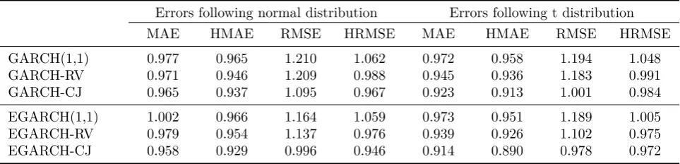
[image:11.595.57.539.274.390.2]

Table 5 below presents the values for out-of-sample forecasting measures. As in in-sample predictive power evaluation, it is found that GARCH-CJ type-models perform better than GARCH-RV and GARCH type-models for predicting future volatility. Also, the EGARCH type-models has smaller measures values than GARCH type-models which supposes that the former have more predictive power. More interestingly, the assumption for normal distribution of errors allows the GARCH type-models to predict better future volatility. This result is not the same for EGARCH type-type-models where predictive power measures are not scattered similarly as for the GARCH type-models, and the predictive power judgment depends also here on the measure used for evaluation.

Table 5: In-Sample Forecast Evaluation

Errors following normal distribution Errors following t distribution MAE HMAE RMSE HRMSE MAE HMAE RMSE HRMSE GARCH(1,1) 0.977 0.965 1.210 1.062 0.972 0.958 1.194 1.048 GARCH-RV 0.971 0.946 1.209 0.988 0.945 0.936 1.183 0.991 GARCH-CJ 0.965 0.937 1.095 0.967 0.923 0.913 1.001 0.984 EGARCH(1,1) 1.002 0.966 1.164 1.059 0.973 0.951 1.189 1.005 EGARCH-RV 0.979 0.954 1.137 0.976 0.939 0.926 1.102 0.975 EGARCH-CJ 0.958 0.929 0.996 0.946 0.914 0.890 0.978 0.972

Our full sample consists of 216,864 observations (5-min returns) corresponding to 1,506 days from January 15, 2010 to January 29, 2016. GARCH and EGARCH type-models are estimated over the first 195,264 observations of the full sample, i.e. over the period January 15, 2010 to June 15, 2015

Based on discussions in sections 3.2.1 and 3.2.2, we conclude that among all the competing models, on top of their best fitting for intraday returns volatility, the GARCH-CJ-type models perform better when forecasting future volatility. Thus, introducing the realized volatility into GARCH model and splitting it into continuous sample path variation (Ct) and discontinuous jumps variation (Jt)

enhances the model’s explanatory and predictive powers.

4 Concluding remarks

In this paper, we constructed a GARCH-CJ type model with continuous sample path variation and discontinuous jump variation based on the GARCH-RV model introduced by Koopman et al. (2005). In order to test the model’s validity, we performed an empirical study using 5-min high-frequency data of the broad based Moroccan All Shares Index (MASI Index) for the period covering January 15, 2010 to January 29, 2016. Then we estimated the parameters of the six competing models, namely, GARCH, GARCH-RV, GARCH-CJ, EGARCH, EGARCH-RV and EGARCH-CJ. We also evaluated each model’s predictive power using a loss function by calculating four measures (MAE, HMAE, RMSE, and HRMSE) in both cases of in-sample and out-of-sample forecasting.

(12)

returns is found to be leptokurtic indicating that volatility is high in the Moroccan stock market. A result that is consistent with other findings of studies on emerging financial markets. Further conclusions are drawn from the estimation results as follows:

(1) The GARCH-type models and EGARCH-type models fit better the data when a Student-t distribution is assumed for residuals ;

(2) Volatility in the Moroccan stock market exhibits pronounced persistence considering the signif-icant positive estimates for introduced realized volatility (RV) ;

(3) The lagged continuous sample path variation contains relatively more information for predicting the current volatility than the lagged discontinuous jump variation ;

(4) According to predictive power of the models, the GARCH-CJ are found to be better than GARCH and GARCH-RV-type models for forecasting future volatility. This result was found when performing both in-sample and out-of-sample forecasting.

These findings mean that it makes sense to split the realized volatility in the GARCH-RV model into a continuous sample path and discontinuous jumps variations to enhance the models explanatory and predictive power of daily volatility in financial practices such as financial derivatives pricing, capital asset pricing, and risk measures.

(13)

References

Andersen, T. G. and Bollerslev, T. (1998). Answering the skeptics: Yes, standard volatility models do provide accurate forecasts. International economic review, pages 885–905.

Andersen, T. G., Bollerslev, T., and Diebold, F. X. (2007). Roughing it up: Including jump compo-nents in the measurement, modeling, and forecasting of return volatility. The Review of Economics and Statistics, 89(4):701–720.

Andersen, T. G., Dobrev, D., and Schaumburg, E. (2012). Jump-robust volatility estimation using nearest neighbor truncation. Journal of Econometrics, 169(1):75–93.

Barndorff-Nielsen, O. E. and Shephard, N. (2006). Econometrics of testing for jumps in financial economics using bipower variation. Journal of financial Econometrics, 4(1):1–30.

Bollerslev, T. (1986). Generalized autoregressive conditional heteroskedasticity. Journal of economet-rics, 31(3):307–327.

Corsi, F. (2009). A simple approximate long-memory model of realized volatility. Journal of Financial Econometrics, page nbp001.

Engle, R. F. (1982). Autoregressive conditional heteroscedasticity with estimates of the variance of united kingdom inflation. Econometrica: Journal of the Econometric Society, pages 987–1007.

Frijns, B., Lehnert, T., and Zwinkels, R. C. (2011). Modeling structural changes in the volatility process. Journal of Empirical Finance, 18(3):522–532.

Fuertes, A.-M., Izzeldin, M., and Kalotychou, E. (2009). On forecasting daily stock volatility: The role of intraday information and market conditions. International Journal of Forecasting, 25(2):259–281.

Huang, C., Gong, X., Chen, X., and Wen, F. (2013). Measuring and forecasting volatility in chi-nese stock market using har-cj-m model. In Abstract and Applied Analysis, volume 2013. Hindawi Publishing Corporation.

Koopman, S. J., Jungbacker, B., and Hol, E. (2005). Forecasting daily variability of the s&p 100 stock index using historical, realised and implied volatility measurements. Journal of Empirical Finance, 12(3):445–475.

Martens, M. (2002). Measuring and forecasting s&p 500 index-futures volatility using high-frequency data. Journal of Futures Markets, 22(6):497–518.