Discretion Rather than Rules? Binding Commitments versus Discretionary Policymaking

Munich Personal RePEc Archive

Discretion Rather than Rules? Binding

Commitments versus Discretionary

Policymaking

Jensen, Christian

Moore School of Business, University of South Carolina

September 2016

Online at

https://mpra.ub.uni-muenchen.de/76838/

Discretion Rather than Rules? Binding

Commitments versus Discretionary Policymaking

Christian Jensen

University of South Carolina

September, 2016

Abstract

Because optimal plans are time-inconsistent, continuing one from a previous period is not optimal from today’s perspective, and may not out-perform discretion, even ignoring gains from surprise deviations. Hence, contrary to conventional wisdom, a binding and credible commitment does not always outperform discretion over time, even if a non-credible com-mitment does. Forward-looking policymakers might therefore not want to irrevocably bind themselves to the optimal plan from any particular period, even if they could. The vast literature proposing different com-mitment mechanisms illustrates that it is a common misconception that a credible commitment to the optimal plan is always preferable to discretion.

JEL Codes: E61; H30; E52

Keywords: Commitment; discretion; policy rules; expectations

∗

1

Introduction

Since the seminal contribution of Kydland and Prescott (1977) showing that the

optimal commitment plan is time-inconsistent (see also Calvo (1978) and Barro

and Gordon (1983a)), so that policymakers have incentives to deviate in any

later period to commit to the new optimal plan, much effort has gone into

ex-ploring ways for policymakers to overcome these incentives, thus enabling them

to credibly commit. For example, policymakers might be able to bind

them-selves to follow the original optimal plan by staking their reputation on it (Barro

and Gordon (1983b) and Rogoff (1987)), by delegating its implementation

(Pers-son and Tabellini (1993), Rogoff (1985), Svens(Pers-son (1997) and Walsh (1995)),

or by making it too time-consuming, or costly, to change course (Kydland and

Prescott (1977) and Kotlikoff, Persson and Svensson (1988)).1

However, these

commitment mechanisms implicitly assume that continuing the original optimal

plan will achieve policymakers’ objectives to a greater extent than discretion also

from the perspective of later periods, making such a commitment desirable also

in the future. We show that this is not always the case.

Because optimal plans are time-inconsistent, continuing the one from a

pre-vious period is not optimal, and as we show, can even do worse than discretion.

Moreover, we show that this is feasible for extremely patient policymakers with

arbitrarily low discount rates, or even completely ignoring any potential gains

from an unanticipated deviation to discretion. Hence, our point is not that the

superiority of commitment over discretion might be insufficient to discourage a

deviation to discretion, and the potential gains from a surprise deviation, but

rather that, from the perspective of future periods, the original optimal

commit-ment plan might simply not be superior to discretion.2

Consequently,

forward-looking policymakers might not want to bind themselves to the optimal plan

from a particular period, even if they could. Our results are relevant in many

policy situations, but especially for monetary policy, where commitment

solu-tions are commonly utilized in normative studies, and sometimes even to guide

actual policy (Dennis (2010)), taking for granted that a binding once-and-for-all

commitment will perform better over time than discretion.

As an example, imagine that the optimal discretionary policy is never to

pun-ish for misbehavior, while the optimal commitment plan calls for punpun-ishing future

misbehavior, so as to discourage it, but not to punish current misbehavior (which

has already taken place, and can therefore not be discouraged). We show that

while always threatening to punish for future misbehavior, but never actually

do-ing so, does better than a policy of never punishdo-ing, as long as the threat remains

credible, always punishing for misbehavior might not do better than never

pun-ishing. In other words, while commitment is always superior to discretion, since

it presumes the benefit of better behavior induced by the threat of punishment

without ever actually incurring the cost of carrying it out, a binding, and thus

credible, commitment, which does require carrying out the punishment to yield

better behavior, might not be superior to discretion. Hence, following through

on rules designed so as to shape expectations of future policy, and thus influence

individuals’ behavior, does not always outperform discretionary policymaking.

In most decision problems, an individual’s optimal present behavior depends

on her expectations about the future, including future policy. As a result, most

policy problems are dynamic, in that the current outcome does not only depend

on the currently implemented policy, but also on that expected to be

imple-mented in the future. The optimal commitment solution exploits these dynamics

by committing to a plan of action for all future periods, chosen so as to shape

expectations optimally from the perspective of the time at which it is designed.

Consequently, from the viewpoint of this original period, it achieves

policymak-ers’ objectives to a greater extent than the optimal discretionary policy, which

does not attempt to influence expectations. However, from the perspective of any

later period, the optimal plan differs, that is, the plan is unchanged in that the

prescribed action to implement xperiods later remains the same, but the action

to implement in a particular period can vary across optimal plans from different

times. Specifically, when the time comes to enforce a previously promised action

designed to influence expectations prior to its implementation, it has already

played its role in terms of shaping these expectations, making it preferable, from

the perspective of the current point in time, to implement the optimal

discre-tionary action. This is why policymakers have incentives to deviate from the

op-timal plan from any previous period, and thus the source of its time-inconsistency.

Policymakers would achieve their objectives to the greatest extent possible

if in every period they could credibly commit to the optimal plan from the

perspective of that period. But, this would, due to time-inconsistency, require

reneging on past commitments in every period, so that these cannot be credible.

has focused on finding ways for policymakers to credibly bind themselves to the

original optimal plan. The idea is that policymakers should ignore the urge to

reoptimize, since credibly recommitting to a new plan in every period is not

fea-sible, and instead remain faithful to the original optimal plan, thus avoiding the

discretionary equilibrium (McCallum (1995), Persson and Tabellini (1994) and

Woodford (1999)). However, while the original plan is preferable to discretion

from the viewpoint of the original starting point, this might not be the case from

the perspective of later periods. If the outdated optimal plan eventually does

worse than the discretionary equilibrium, how can the original commitment to

follow this plan in all future periods be credible? Since bygones are bygones,

the fact that the original plan did better initially is irrelevant, and policymakers

would prefer to divert to the discretionary equilibrium. If, instead, the original

plan does better over time than discretion, the implicit threat of diverting to the

less desirable discretionary equilibrium can motivate policymakers to overcome

the temptation to deviate.

We assume a strict trigger-strategy where the public comes to expect

dis-cretion in all periods following any deviation from a previous commitment, no

matter what policymakers say or do (Chari and Kehoe (1990)). Combined with

rational expectations, this implies that policymakers must choose between the

original optimal plan and the discretionary equilibrium, there is no other option.

Because credibly committing to a new plan in every period is not feasible, the fact

that doing so would yield better results than remaining faithful to the original

optimal plan is irrelevant. What matters then is whether a binding commitment

to the original plan yields better results over time than discretion, the only

strategy of reverting to discretion forever is, or how the public would coordinate

on it. On one hand policymakers have incentives to mislead the public, as

dis-cussed above, by promising to follow the optimal plan in the future, but then

implementing the optimal discretionary policy. On the other hand, individuals

have incentives to forecast future policy as accurately as possible, assuming

fore-cast errors lead to suboptimal decisions. Hence, if policymakers were to return to

the old commitment plan after a deviation, it would be in individuals best interest

to adapt their expectations, if it enables them to forecast better. Of course, the

more severe and credible the punishment for deviating from past commitments

is, the more it deters these (al-Nowaihi and Levine (1994)).

Each of the three sections below studies a model where continuing the

op-timal plan from a previous period can lead to worse outcomes than discretion.

The first is a stylized model, which while not very realistic, provides the clearest

illustration. The second example is a standard new-Keynesian sticky-price model

of the inflation-output trade-off, commonly used to analyze and guide monetary

policy. The last example is a more general model, where the problem is

attenu-ated.3

The more distant the policy expectations affecting the current state, the

more prone the old optimal plan is to being outperformed by discretion.

3

2

Stylized model

Imagine a policy problem for which in any period t0 the objective is to minimize

Et0

∞

X

t=t0

βt−_t0

π2_t +ωy_t2 (1)

subject to

πt=βJEtπt+J +αyt+ut (2)

for t = t0, t0+ 1, t0+ 2, . . . where β ∈ (0,1), ω > 0, α > 0, and J is an integer

greater or equal to one. The constraint (2) links the policy instrument πt to the

endogenous variable yt, which also depends on the exogenous stochastic shock

ut and period-t expectations of the policy to be implemented J periods later,

Etπt+J.

Exploiting that certainty equivalence prevails in this linear-quadratic

frame-work (Currie and Levine (1993, pp. 95-121)), the optimal commitment policy

can be obtained by inserting the constraint (2) into the objective (1), ignoring

the expectations operator, and minimizing the resulting sum

∞

X

t=t0

βt−_t0

π2_t + ω

α2 πt−β

J_π

t+J−ut

2

(3)

with respect to the policy instrument {πt}∞t=t0. The corresponding first-order

conditions yield

πt=− ω

for t=t0, t0+ 1, t0+ 2, . . . , t0+J −1, and

πt=− ω αyt+

ω

αyt−J (5)

for t = t0 +J, t0 +J + 1, t0 +J + 2, . . ., the optimal commitment plan from

the perspective of any period t0. This plan is time-inconsistent, because if the

policy problem were reconsidered in any later period t′

0 > t0, the optimal plan

would differ, prescribing equation (4) in periods t′

0, t

′

0 + 1, t

′

0 + 2, . . . , t

′

0 +J −1

and equation (5) in t=t′

0+J, t

′

0+J+ 1, t

′

0+J+ 2, . . ., as this would minimize

Et′

0

∞

X

t=t′

0

βt−t′

0 π2

t +ωy

2

t

, (6)

the period-t′

0policy objective. The optimalt

′

0-plan postpones the implementation

of equation (5) relative to the optimal plan from period t0. The reason is that

according to the constraint (2), only expectations of policy J periods into the

future matter for the current state, and when policymakers reoptimize at any

later time, J periods into the future gets pushed further ahead. When the policy

problem is reconsidered in every period, policymakers always implement equation

(4), which constitutes the optimal discretionary policy.

The value of the policy objective (1) in any period t0 depends not just on

the policy applied in t0, but also on that expected to be implemented in all

subsequent periodst0+ 1, t0+ 2, t0+ 3, . . . This is what the optimal commitment

solution exploits to outperform the discretionary one. Over time, the best possible

outcome for policymakers arises when they can commit in each period to the

equation (4) in every period, while simultaneously convincing people that they

will switch to equation (5) J periods later. Of course, continuously promising a

policy switch in the future that gets pushed off in the subsequent period, cannot

be credible. Sooner or later the public would realize that the switch will never

happen, and come to expect equation (4) to be implemented in all future periods.

As a result, we would go from the commitment solution to the discretionary one.

Ruling out the possibility of systematically misleading the public period after

period, focus has been on finding ways for policymakers to credibly commit to

the original optimal plan, thus avoiding the discretionary equilibrium. What we

ask is whether it is desirable to bind oneself to the original optimal plan, i.e., is it

superior to discretion over time? The discretionary solution matches the optimal

plan from the perspective of period t0 for t = t0, t0 + 1, t0 + 2, . . . , t0 +J −1,

but deviates from it for t = t0 +J, t0+J+ 1, t0+J+ 2, . . . The optimal plan

from t0 −1 matches that from t0 for all periods except t0+J−1. The optimal

plan from t0 − 2 matches that from t0 in all periods except t0 + J − 1 and

t0+J−2. Any optimal plan fromt0−J or earlier deviates from the one fromt0 for

t =t0, t0+1, t0+2, . . . t0+J−1, but matches it fort=t0+J, t0+J+1, t0+J+2, . . .

Hence, the old plan deviates more the more outdated it is, and the larger is J.

Given that a credible, once-and-for all, commitment would eventually require

implementing the optimal plan from more than J periods ago, how will that

compare with the optimal discretionary policy from the perspective of the policy

objective in that future period? Assuming that the plan originated int0, and that

t′

0 is any period such that t

′

0 ≥t0+J, continuing the original commitment plan

would require implementing equation (5) in all periods t′

0, t

′

0+ 1, t

′

0+ 2, . . . that

are relevant for the period-t′

depend on the initial conditions y_t′

0−J, yt′0−J+1, yt′0−J+2, . . . , yt′0−1 and ut′0, which are unknown at time t0, and would vary with the choice of t

′

0. 4

Integrating the

policy objective (6) over all feasible initial conditions, yields

E

∞

X

t=t′

0

βt−_t′

0 π2

t +ωy

2

t

, (7)

the unconditional loss function. While policymakers can use current conditions to

predict future initial conditions, looking far enough ahead, which is necessary due

to the once-and-for-all nature of the optimal commitment policy, these become

irrelevant, and the pertinent objective is the unconditional expected value of

the loss.5

Its value when continuing the optimal plan from period t0, enforcing

equation (5) in all periods t=t′

0, t

′

0+ 1, t

′

0+ 2, . . ., is

Lc =

8ω3

β2J _ωp−α2 ρJ(α2

−r)

s

(ω(1 +βJ_(1−2ρJ_{)) +α}2_+r)2_(2ωβJ _−ρJ_{(ω(1 +β}J_{) +α}2_−r))q (8)

where

s = σ

2

(1−ρ2_{) (1−β)}, (9)

p= 2ω 1−βJ

1−ρJ

+α2 2 1−βJ

−ρJ βJ + 3

+ 2r ρJ −1

, (10)

q =ω 1 +βJ ω 1−βJ+ 2α2−r+α2 α2−r, (11)

r = q

ω2_(1−βJ₎2_+α2_(α2_{+ 2ω(1 +β}J_{)), (12)}

4

If initial conditions yt′

0−J, yt′0−J+1, yt′0−J+2, . . . , yt′0−1 all equal zero, the optimal

commit-ment plan from t0 would implement the exact same conditions as the optimal plan from t ′ 0, and cannot be improved upon. However, given the stochastic shock ut, this is highly unlikely,

especially for largeJ. 5_{This exploits that E}

t0

P∞

t=t′

0β

t−t′ 0(π2

t+ωy

2

t) =E

P∞

t=t′

0β

t−t′ 0(π2

t +ωy

2

t) for large enough

t′

5 10 15 20 25 30 .05

.10 .15 .20 .25 .30 .35

ω α

J=1 J=2 J=3 J=4 J=5 J=6 J=7 J=8

J=12 J=16

J=32

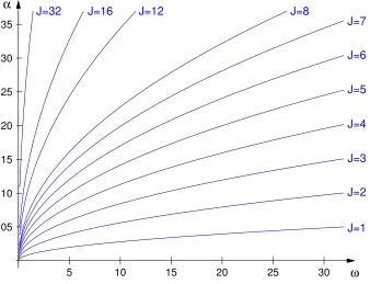
Figure 1: Old commitment plan vs. discretion, Lc =Ld.

assuming a persistent shock

ut=ρut−1+at (13)

where a_t is white noise with variance σ2

and ρ ∈ (0,1). When the optimal

discretionary policy (4) is implemented in all periods t=t′

0, t

′

0+ 1, t

′

0+ 2, . . ., its

value is

Ld=

ω(ω+α2

)s

(ω(1−βJ_ρJ_{) +α}2₎2. (14)

Assumingβ =.99 andρ=.9, figure 1 plots iso-loss curves for different values

ofJ, that is, combinations ofαandωfor whichLd =Lc, so that the expected loss

(7) is the same for optimal discretion and any optimal commitment plan that is

at least J periods old.6

For each of the curves, and corresponding value of J, the

optimal commitment plan fromt0 does better than discretion for combinations of

α and ω above the curve, and worse than discretion for parameter combinations

below the curve. As is evident from the figure, it is possible for discretion to do

better, on average, than the optimal plan from t0. In particular, this is more

prone to occurring, the larger J is. The reason is, as discussed above, that

from the perspective of the period-t′

0 objective (6), the commitment plan from

t0 implements a suboptimal equation in the first J periods, implementing the

optimal one after that, while discretion implements the optimal equation in the

first J periods, implementing a suboptimal one afterwards. Hence, the larger

J is, the greater the advantage of discretion over the optimal commitment plan

from t0, and the larger the set of parameter values for which it dominates.7

The assumed trigger strategy requires that the discretionary solution (4)

per-tain in all periods following a deviation from previous commitments.

Conse-quently, if policymakers deviate from the optimal t0-plan in any later period t

′

0,

the policy objective (6) would on average take the value Ld from then on. If

instead they remain truthful to the optimal t0-plan, the policy objective would

on average take the value Lc. Looking forward, predicting whether policymakers

will want to deviate from the once-and-for-all commitment to the optimalt0-plan

section). Lowering β rotates the curves up around their intercept on theα-axis, making the area where discretion dominates larger. Raising β has the opposite effect, as does lowering

ρ. The standard deviation σ has no impact on Lc/Ld, or the figure. Estimates of α and

ω for the monetary policy model vary across studies and countries, with α ∈ (.001, .37) and

ω ∈(.001,31.37), see Assenmacher-Wesche (2006), Dennis (2004), Givens (2012), Schorfheide (2008), and S¨oderstr¨om, S¨oderlind and Vredin (2005). Most studies find parameter values to-wards the lower ends. While these values are not necessarily relevant forJ 6= 1, or outside the New-Keynesian model, we use these as a benchmark throughout.

7_{A similar figure can be computed comparing the two policies from the perspective} of the conditional objective (6). It would be sensitive to the assumed initial conditions

yt′

0−J, yt′0−J+1, yt′0−J+2, . . . , yt′0−1 and ut′0, but unless these are all zero, it remains true that

in any later period t′

0 far enough into the future (so that the unconditional

ob-jective becomes relevant), depends on Ld and Lc. If Ld < Lc, policymakers will

eventually want to deviate from the optimal t0-plan because it would eventually

do worse, on average, than discretion, from the perspective of expected future

policy objectives (6). The fact that the t0-plan did better than discretion

orig-inally, would be irrelevant, as bygones are bygones. If Ld > Lc, policymakers

might not want to deviate from the optimal t0-plan, as it does better, on

aver-age, than the only viable alternative, the discretionary equilibrium. Moreover,

the implicit threat of ending up at the inferior discretionary equilibrium might

act as a deterrent to deviating. However, Ld > Lc is insufficient to guarantee

that policymakers would not deviate from the original optimal plan, since there

can be additional gains from an unanticipated deviation. If large enough, these

gains might more than compensate for any expected future gains from remaining

faithful to the original optimal plan, especially for impatient policymakers.

Contrary to Taylor (1979a), Woodford (1999, 2003) and Jensen and

McCal-lum (2010), we are not suggesting that policymakers should ignore present initial

conditions when evaluating different policies. Also, our point is not that once

outdated, the original optimal plan can do worse than discretion from an

un-conditional point of view, but that looking forward, it would be expected to

eventually do worse, on average, in terms of the original conditional objective.

Since bygones are bygones, policymakers would then want to deviate from the

original plan, despite knowing that they would never be able to commit again

(due to the assumed trigger strategy). That is, they would from then on prefer

the discretionary equilibrium in all future periods rather than maintaining a

surprise deviation. Hence, they would not deviate in an attempt to commit to

the new optimal plan, which is by assumption unfeasible, but rather to settle on

the discretionary equilibrium.

3

Contemporary model

The New-Keynesian sticky-price model of the inflation-output trade-off is

exten-sively used to study monetary policy. In its simplest version, it is identical to

the model above when J = 1, πt denotes inflation and yt is output, both

mea-sured in terms of period-t deviations from their respective flexible-price values.

The variable ut is a cost-push shock. The policy objective (1) is derived as a

quadratic approximation to a representative household’s expected life-time

util-ity in periodt0, so in each period, policymakers seek to maximize the discounted

sum of households’ present and expected future utility. The parameters αand ω

depend on the degree of price-stickiness, while β is a discount factor.8

Since J = 1, continuing the optimal plan from any previous period t0 in

any later period t′

0 > t0 only deviates from the optimal t

′

0-plan in terms of the

action implemented in t′

0, equation (5) instead of (4). The impact this has on

the t′

0 policy objective (6) depends on the conditions that happen to prevail at

the time (Dennis (2001, 2010)). When y_t′

0−1 = 0, the optimal plan from any previous period is identical to that from t′

0, and cannot be improved upon. The

moreyt′

0−1 differs from zero, the more the implemented action (5) differs from the

optimal one (4), and the less desirable the objective value (6) becomes. The

dis-cretionary solution only matches the optimalt′

0-plan in terms of the initial-period

action, differing in all later periods. Hence, from the perspective of any period

t′

0, whether the discretionary solution does better or worse than any optimal plan

from the past, depends on the initial condition yt′

0−1. As initial conditions vary over time, whether discretion or the outdated plan is preferable, will also vary.

But, integrating over these initial conditions, as above, figure 1 shows that even

in this case (J = 1), discretion can, on average, do better than an outdated

opti-mal commitment plan, despite doing worse for most parameter values.9

It is just

that when J = 1, the expectational dynamics are so simple that it is difficult for

discretion to outdo the outdated optimal plan, since the latter only differs from

the updated optimal plan in the initial period.

4

More general models

The simple expectational dynamics in current and past policy models,

exempli-fied in the previous section, favor a credible once-and-for-all commitment over

discretion. However, there are examples, beyond the stylized one in the second

section, of relevant models that are less favorable to commitment. Replacing the

constraint above (2) with

πt = J

X

j=1

βjEtπt+j +αyt+ut, (15)

9

yields a model with more complicated, and maybe more realistic, expectational

dynamics, where expectations about policy in allJ future periods are relevant,

in-stead of just in one particular future period. Keeping the objective (1) unchanged,

the optimal commitment plan from the perspective of period t0 becomes

πt0 =−

ω

αyt0 (16)

πt0+1 =−

ω

αyt0+1+

ω

αyt0 (17)

πt0+2 =−

ω

αyt0+2+

ω

αyt0+1+

ω

αyt0 (18)

...

πt =− ω αyt+

ω αyt−1+

ω

αyt−2+· · ·+ ω

αyt−J (19)

where the latter equation (19) applies for t=t0+J, t0+J+ 1, t0+J+ 2, . . . In

this case, the optimal plan prescribes a different policy equation for each of the

initialJ periods, so continuing the optimal plan from any earlier time implements

a suboptimal equation in the firstJ periods. The discretionary solution matches

the currently optimal plan only in the initial period. Which does better, the old

plan or discretion, again depends on how outdated the old plan is, the conditions

that happen to prevail at the time, and the parameter values, in particular J.

However, these more complicated expectational dynamics illustrate more clearly

how the optimal plan from a previous period fails to shape expectations of future

policy optimally from the perspective of the present period, thus making it more

prone to doing worse than discretion, which makes no attempt at influencing

expectations.

policy problems has been suggested in the literature, at least for monetary policy,

arising with alternative models of price-setting, for example with multi-period

Taylor (1979b) contracts, or for Calvo-pricing with time-varying trend inflation

(Sbordone (2007)). Another example is the sticky-information model (Mankiw

and Reis (2002)), where the Phillips curve constraint is

πt= J

X

j=1

bjEt−j(πt+cyt) +ayt+ut (20)

with strictly positive b1, b2, . . . , bJ, c and a, where J is a strictly positive

inte-ger denoting the maximum number of periods producers go without updating

their information sets. While the timing of the policy expectations differ,Et−jπt

instead of Etπt+j, the commitment solutions are similar in that the optimal t0

-plan implements discretion int0, but proposes gradually more complicated policy

equations for t0+ 1 throught0+J, as it takes into account the effects policy

ex-pectations have on thet0-policy objective (1), which are more complex the longer

ahead the policy is known (up to J).

5

Conclusions

Optimal plans are time-inconsistent, so continuing the one from a previous

pe-riod is not optimal from today’s perspective, and can do worse, we show, in terms

of achieving policymakers’ contemporary objectives, than the discretionary

equi-librium. Thinking ahead, policymakers might therefore not wish to irreversibly

commit to the optimal plan from any given period, even if they could, but

that whether or not a binding commitment is desirable, depends on the policy

problem at hand. In particular, it depends on how complicated the expectational

dynamics are, especially how long it takes for the optimal plan to settle on a

particular policy action, but can even vary with the parameter values.

6

References

al-Nowaihi, A. and Levine, P. (1994) “Can Reputation Resolve the Monetary Policy Credibility Problem?” Journal of Monetary Economics 33: 355-380.

Atkeson, A. and Lucas, R. (1992) “On efficient distribution with private in-formation.” Review of Economic Strudies 59: 427-453.

Assenmacher-Wesche, K. (2006) “Estimating Central Banks preferences from a time-varying empirical reaction function.” European Economic Review 50: 1951-1974.

Barro, R. J. and Gordon, D. B. (1983a) “A Positive Theory of Monetary Policy in a Natural Rate Model.” Journal of Political Economy 91: 589-610.

Barro, R. J. and Gordon, D. B. (1983b) “Rules, discretion and reputation in a model of monetary policy.” Journal of Monetary Economics 12: 101-121.

Blake, A. P. (2001) “A ‘timeless perspective’ on optimality in forward-looking rational expectations models.” Working paper, NIESR.

Calvo, G. A. (1978) “On the Time Consistency of Optimal Policy in a Mon-etary Economy.” Econometrica 46: 1411-1428.

Calvo, G. A. (1983) “Staggered Prices in a Utility Maximizing Framework.”

Journal of Monetary Economics 12: 383-398.

Chari, V. V. and Kehoe, P. J. (1990) “Sustainable Plans,”Journal of Political Economy 98: 783-802.

Clarida, R., Gali, J. and Gertler, M. (1999) “The science of monetary policy: A new Keynesian perspective.” Journal of Economic Literature 37: 1661-1707.

Currie, D. and Levine, P. (1993)Rules, Reputation and Macroeconomic Policy Coordination, Cambridge University Press.

policymak-ing from behind a veil of uncertainty.” Workpolicymak-ing paper, Federal Reserve Bank of San Francisco.

Dennis, R. (2004) “Inferring Policy Objectives from Economic Outcomes.”

Oxford Bulletin of Economics and Statistics 66: 735-764.

Dennis, R. (2010) “When is discretion superior to timeless perspective poli-cymaking?” Journal of Monetary Economics 57: 266-277.

Givens, G. E. (2012) “Estimating Central Bank Preferences under Commit-ment and Discretion.” Journal of Money, Credit and Banking 44: 1033-1061.

Green, E. (1987) “Lending and the smoothing of uninsurable income” In

Contractual arrangements for intertemporal trade, edited by Prescott, E. and

Wallace, N. University of Minnesota Press.

Jensen, C. (2001) “Optimal Monetary Policy in Forward-Looking Models with Rational Expectations.” Working paper, Carnegie Mellon University.

Jensen, C. and McCallum, B. T. (2010) “Optimal Continuation versus the Timeless Perspective in Monetary Policy.” Journal of Money, Credit and Banking

42, 1093-1107.

King, R. G. and Wolman, A. (1999) “What Should the Monetary Authority Do When Prices Are Sticky?” In Monetary Policy Rules, edited by Taylor, J. B. University of Chicago Press: 349-404.

Kotlikoff, L. J., Persson, T. and Svensson, L. E. O. (1988) “Social Contracts as Assets: A Possible Solution to the Time-Consistency Problem.”, American Economic Review 78: 662-677.

Kydland, F. E. and Prescott, E. C. (1977) “Rules Rather than Discretion: The Inconsistency of Optimal Plans.” Journal of Political Economy 85: 473-492. Mankiw, N. G. and Reis, R. (2007) “Sticky Information in General Equilib-rium.” Journal of the European Economic Association 5: 603-613.

McCallum, B. T. (1995) “Two Fallacies Concerning Central-Bank Indepen-dence.” American Economic Review 85: 207-211.

Persson. T. and Tabellini, G. (1993) “Designing institutions for monetary stability.” Carnegie-Rochester Conference Series on Public Policy 39: 53-84.

Persson. T. and Tabellini, G. (1994) Monetary and fiscal policy - Volume I: Credibility. MIT Press.

Journal of Economic Theory 79: 174-191.

Rogoff, K. (1985) “The Optimal Degree of Commitment to an Intermediate Monetary Target.” Quarterly Journal of Economics 100: 1169-1189.

Rogoff, K. (1987) “Reputational Constraints on Monetary Policy.” Carnegie-Rochester Conference Series on Public Policy 26: 141-82.

Rotemberg, J. J. (1982) “Monopolistic Price Adjustment and Aggregate Out-put.” Review of Economic Studies 49: 517-531.

Rotemberg, J. J. and Woodford, M. (1999) “Interest Rate Rules in an Esti-mated Sticky Price Model.” In Monetary Policy Rules, edited by Taylor, J. B. University of Chicago Press: 57-126.

Sbordone, A. M. (2007) “Inflation Persistence: Alternative Interpretations and Policy Implications.” Journal of Monetary Economics 54: 1311-1339.

Schorfheide, F. (2008) “DSGE Model-Based Estimation of the New Keynesian Phillips Curve.” Federal Reserve Bank of Richmond Economic Quarterly 94: 397-433.

Sleet, C. and Yeltekin, S. (2005) “Credible Social Insurance.” Working paper, Carnegie Mellon University.

S¨oderstr¨om, U., S¨oderlind, P. and Vredin, A. (2005) “New-Keynesian Models and Monetary Policy: A Re-examination of the Stylized Facts.” The Scandina-vian Journal of Economics 107: 521-546.

Stokey, N. (1991) “Credible public policy.” Journal of Economic Dynamics and Control 15: 367-390.

Svensson, L. E. O. (1997) “Optimal Inflation Targets, ‘Conservative’ Central Banks, and Linear Inflation Contracts.” American Economic Review 87: 98-114. Svensson, L. E. O. and Woodford, M. (2002) “Indicator Variables for Optimal Policy.” Journal of Monetary Economics 50: 691-720.

Svensson, L. E. O. and Woodford, M. (2005) “Implementing Optimal Policy through Inflation-Forecast Targeting.” InThe Inflation-Targeting Debate, edited by Bernanke, B. S. and Woodford, M. University of Chicago Press: 19-92.

Taylor, J. B. (1979a) “Estimation and control of a macroeconomic model with rational expectations.” Econometrica 47: 1267-1286.

Thomas, J. and Worrall, T. (1990) “Income fluctuation and asymmetric infor-mation: an example of a repeated principal-agent problem.” Journal of Economic Theory 51: 367-390.

Woodford, M. (1999) Commentary: How Should Monetary Policy Be Con-ducted in an Era of Price Stability. In New Challenges for Monetary Policy.

Federal Reserve Bank of Kansas City: 277-316.

Woodford, M. (2000) “Pitfalls of Forward-Looking Monetary Policy.” Amer-ican Economic Review 90: 100-104.