A topological approach to structural change analysis and an application to long run labor allocation dynamics

Munich Personal RePEc Archive

A topological approach to structural

change analysis and an application to

long-run labor allocation dynamics

Stijepic, Denis

Fernuniversität in Hagen

9 October 2016

Online at

https://mpra.ub.uni-muenchen.de/74568/

1

A TOPOLOGICAL APPROACH TO STRUCTURAL CHANGE ANALYSIS AND AN APPLICATION TO LONG-RUN LABOR ALLOCATION DYNAMICS

Denis Stijepic*

Fernuniversität in Hagen

October 2016

Abstract. A great part of economic literature deals with structural changes, i.e. long-run changes in

the structure of economic aggregates. While the standard literature relies on the mathematical

branches of analysis and algebra for modeling structural change and describing the relevant empirical

evidence, we choose a topological approach, which relies on the notions of self-intersection and

mutual intersection of trajectories. We discuss all the methodological and mathematical aspects of this

approach and show that it is applicable to a wide range of classical topics and papers of growth and

development theory. Then, we apply it for studying a specific type of structural change, namely, the

long-run labor re-allocation across sectors: we (a) elaborate new empirical evidence stating that

mutual intersection and non-self-intersection are stylized facts of long-run labor re-allocation, (b)

suggest and discuss theoretical explanations of non-self-intersection, and (c) discuss mathematical

methods for explaining mutual intersection by using standard structural change models. Overall, our

approach generates new evidence, new critique points of the previous structural change literature, new

theoretical arguments, and a wide range of new research topics.

JEL Codes. C61, C65, O41

Keywords. Structural change, dynamics, long run, trajectory, intersection, self-intersection,

differential equations, geometry, topology, labor, allocation, savings, functional income distribution.

_______________________

2 1. INTRODUCTION

Structural change, i.e. long-run change in the structure of economic aggregates1 (such as

GDP, aggregate employment, aggregate income, aggregate consumption expenditures), is a

central aspect of growth and development theory2 and has been analyzed in numerous models

and empirical studies over the last centuries.3 While the standard literature relies on the

mathematical branches of analysis and algebra for modeling structural change and describing

the relevant empirical evidence, we suggest a topological approach for studying structural

change.

The first part of our paper deals with the conceptual, methodological, and mathematical

aspects of the topological approach. As discussed there, structural change (in a country) can

be described by a trajectory on the standard simplex, where the trajectories (of different

countries) can be characterized by the topological notions of self-intersection and (mutual)

intersection. Thus, empirical evidence and (existing) theoretical models can be classified by

using these notions; moreover, the models can be compared with the empirical evidence on

(self-)intersection. We discuss the two key aspects of this comparison: the type of economic

law that the models represent (cf. Section 4.2.4) and the different ways to generate

(non-)(self-)intersecting (families of) trajectories in continuous dynamical systems (cf. Section

5.2), where we focus on differential equation systems for discussing the latter aspect. The

definition of structural change and the topological approach developed in the first part of our

paper are relatively general and cover many core topics (among others, savings rate

dynamics, functional income distribution, personal wealth distribution, and cross-sector labor

re-allocation) and classical literature contributions of growth and development theory (cf.

Section 2.2). In general, the topological approach proves useful for studying lower

dimensional structures (e.g. three-sector models), i.e. structures representable on two- and

one-dimensional simplexes, since in this case, it is relatively simple to identify the points of

(self-)intersection in empirical data (cf. Section 3.4).

In the second part of our paper, we demonstrate how to apply the topological approach

developed in the first part of our paper. Due to space restrictions, we focus on a specific sort

of structural change, namely, the long-run labor re-allocation in the three-sector framework

1

Every aggregate index can be divided into its components. Then, the contribution of the components to the aggregate index (i.e., the components’ shares in the aggregate index) can be calculated. In our paper, structural change refers to the long-run dynamics of these contributions/shares. For a formal definition of the term “structural change”, see Section 2.1.

2

For various examples of topics and papers that are covered by our structural change definition, see Section 2.2.

3

3

referring to the agricultural, manufacturing, and services sector. To demonstrate how to use

the topological approach to derive stylized facts, we analyze the data on the long-run labor

allocation dynamics in the OECD countries and formulate two new stylized facts stating that

(a) the labor allocation trajectories intersect mutually in the long run and (b) self-intersection

seems to be a short-run phenomenon and, thus, non-self-intersection is characteristic for the

long run. To demonstrate how use the topological approach to classify theoretical models and

compare them with empirical evidence, we study the Kongsamut et al. (2001) model (which

is a major example of the modern labor re-allocation literature) and discuss under which

(parameter) conditions it can generate (self-)intersections.

Since we are not aware of any literature that discusses or tries to theoretically explain the

stylized facts derived in the second part of our paper,4 we devote the third part of our paper to

this topic. While (mutual) intersections seem to be easily explainable by cross-country

parameter variation and parameter perturbations (cf. Section 5.2.1), the long-run

non-self-intersection seems to be an interesting theoretical puzzle. Therefore, we focus on it and

elaborate different theoretical and intuitive/economic explanations of non-self-intersection of

the long-run labor re-allocation trajectories and of the trajectories associated with some other

topics (cf. Section 2.2) covered by our approach. In part, we discuss these aspects by relying

on topological concepts (in particular, homeomorphisms).

As a byproduct of the main discussion, our paper provides (a) an overview and discussion of

the applicability of different mathematical dynamic models (parameter perturbations, smooth

autonomous differential equations, non-autonomous differential equation systems, coverings,

homeomorphisms, etc.) in structural change modeling and (b) a classification of various

central topics of growth and development theory under the headline of structural change.

Overall, our approach generates new evidence, new critique points of the previous structural

change literature, new theoretical arguments, and numerous topics for further research (which

are summarized in Section 9).

The rest of the paper is set up as follows. The first part of our paper encompasses Sections

2-5. In Section 2, we define the term “structural change” and provide examples of topics and

literature covered by this definition. Section 3 explains the geometrical interpretation of

structural change and the topological classification of structural trajectories. Section 4

4

4

discusses the methodological aspects of the theoretical explanation of trajectory-related

empirical evidence. Section 5 joins these methodological results with some standard results

of the mathematical differential equation theory to elaborate approaches for explaining the

observed (self-)intersection of structural change trajectories by using standard structural

change models (which are representable by differential equation systems). The second part of

our paper encompasses Sections 6 and 7. In Section 6, we present the evidence on labor

re-allocation focusing on OECD countries and the data from The WorldBank and Maddison

(1995, 2007) and formulate the stylized facts regarding the topological properties of labor

allocation trajectories. Section 7 discusses the Kongsamut et al. (2001) model. The third part

of our paper (Section 8) is devoted to the development of a theoretical intuitive/economic

explanation of non-self-intersection. A summary of our findings and a discussion of the

topics for further research are provided in Section 9.

2. A MATHEMATICAL DEFINITION OF STRUCTURAL CHANGE AND EXAMPLES OF TOPICS/LITERATURE COVERED BY IT

We suggest mathematical definitions of the terms “structure” and “structural change” in

Section 2.1 and discuss various examples of topics and classical growth and development

theory papers covered by these terms in Section 2.2.

2.1 Mathematical Definition of Structure and Structural Change

Let y denote an aggregate index (e.g. aggregate employment). Every aggregate index can be

divided into its components (e.g. employment in agriculture, employment in manufacturing,

and employment in services), such that that it is equal to the sum of its components. Let y1,

y2,…yn be the components of the index y. Thus, y = y1 + y2 +…yn (e.g. aggregate

employment = employment in agriculture + employment in manufacturing + employment in

services).

The importance of a component yi (where i

∈

(y) can be measured by the share yi/y (e.g. the importance of agricultural employment with

respect to aggregate employment can be indicated by the

agricultural-employment-to-aggregate-employment ratio, i.e. the agricultural employment share). Let xi denote the share

of component yi in the aggregate index y, i.e. xi:= yi/y for i = 1,2,…n. Note that x1 + x2 +…xn

= 1, since y1 + y2 +…yn = y. Furthermore, we consider here only the economic variables (yi)

that cannot be negative; thus, xi≥0 for i = 1,2,…n. (For example, employment shares cannot

5

We define the term “structure (of the index y)” such that it refers to the tuple (x1,x2,…xn). In

other words, the “structure (of the index y)” is given by the shares of the index components in

the index. (For example, the structure of employment in our example is given by the tuple of

three numbers: agricultural employment share, manufacturing employment share, and

services employment share.) In general, the term “structural change” (as it is used in the

economic literature) refers to the long-run changes in the structure of some aggregate index

(cf. Footnote 1). Thus, according to our definition of the term “structure”, “structural

change” means that at least some of the shares x1, x2,…xn are not constant in the long run.

For example, x1 may grow over time, x2 may decline over time, x3 may decline over time, x4

may be constant over time,…xn may grow over time.

Definitions 1 and 2 summarize this discussion, where we do not implement the facts that

structural change refers to the long run and that we focus on low-dimensional structures (cf.

Section 1), since in this way the mathematical formulations are simpler (we do not need a

mathematical definition of the long run) and more general (i.e. referring to higher dimension).

However, whenever the time frame and dimension become relevant (e.g. in Section 6) we

take account of them.

Definition 1. Let y be an aggregate index and y1, y2, …yn be the components of the index,

where n is a natural number. Let y(t) and y1(t), y2(t),…yn(t) denote the values of the index y

and its components y1, y2, …yn at time t, respectively, where t∈D⊆R and R is the set of real

numbers. Define xi(t):= yi(t)/y(t) ∀t∈D ∀i∈{1,2,…n}. The “(n-dimensional) structure” (of

the index y) at time t∈D is represented by the vector X(t):= (x1(t),x2(t),…xn(t))∈Rn, where

X(t) satisfies the following conditions

(1) ∀t∈D∀i∈

{

}

(2) ∀t∈D x₁(t)+x₂(t)+...+xn(t)=1.

Thus, Definition 1 states that an n-dimensional structure (of the index y) is simply a vector in

n-dimensional real space that satisfies the conditions (1) and (2). Structures, as defined in

Definition 1, are often used in economics. In particular, Definition 1 covers many standard

6

Definition 2. Structural change (over the period [a,b]) refers to the change (or: dynamics)

of X(t) (over the period [a,b]); cf. Definition 1. In particular, the structure has changed over

the period [a,b], if ∃t∈(a,b] X(t)≠X(a).

Simply speaking, Definition 2 states that structural change takes place if X(t) is not constant.

2.2 Examples of Topics and Literature Covered by Definition 2

Since the discussion in Section 2.1 seems quite abstract, we provide now some examples of

topics and structural change literature covered by Definition 2. In this way, we can give our

structural change definition an intuitive/economic meaning and, thus, facilitate the

understanding of the rest of the paper and, in particular, of Sections 3-5. We have tried to

choose the topics of Examples 1-8 such that the significance of structural change (as defined

in Definition 2) as a core topic of growth and development theory is emphasized. Due to this

significance, we have chosen Definition 2 over the many alternative structural change

definitions5 as the basis for our topological approach to structural change analysis. Note that

we refer to Examples 1-8 throughout the paper and, in particular, in Section 8 (for elaborating

a theoretical explanation of non-self-intersection). Furthermore, the topics discussed in

Examples 1-8 imply in association with the results of our paper numerous topics for further

research, e.g. testing for (self-)intersection of trajectories in each field of literature discussed

in Examples 1-8. For these reasons, it makes sense to explain the examples carefully.

Example 1. One of the most obvious application fields of Definition 2 is the literature on

long-run labor re-allocation in multi-sector growth models, e.g. Kongsamut et al. (2001),

Ngai and Pissarides (2007), Foellmi and Zweimüller (2008), and Herrendorf et al. (2014).

These models can be represented here by the following assumptions: li(t) stands for the

employment in sector i at time t, where i = 1,2,…n; l(t):= l1(t) + l2(t) +…ln(t) is the aggregate

employment; xi(t):= li(t)/l(t) is the employment share of sector i at time t and, thus, X(t)≡

(x1(t),x2(t),…xn(t)) indicates the cross-sector labor allocation at time t. Obviously, these

assumptions imply that the cross-sector labor allocation X(t) satisfies conditions (1) and (2)

(among others since employment cannot be negative) and is, therefore, a “structure”

according to Definition 1. Finally, Definition 2 states that structural change takes place if the

labor allocation X(t) changes over time. That is, structural change refers here to cross-sector

5

7

labor re-allocation. Thus, we have shown that the long-run labor re-allocation models are

covered by Definition 2.

Example 2. The three-sector framework is a well-known special case of Example 1. Most of

the papers (e.g. Kongsamut et al. (2001), Ngai and Pissarides (2007), and Foellmi and

Zweimüller (2008)) refer in some way to this framework. We obtain the three-sector

framework if we assume in addition to the assumptions made in Example 1 that: n = 3, i.e.

there are only three sectors; sector 1 (i = 1) represents the primary/agricultural sector, sector 2

(i = 2) represents the secondary/manufacturing sector, and sector 3 (i = 3) represents the

tertiary/services sector. Then, it follows immediately that: X(t) represents the labor allocation

across agriculture, manufacturing, and services at time t; X(t) is a structure, i.e. satisfies (1)

and (2); changes in X(t), i.e. labor re-allocation across agriculture, manufacturing, and

services, represent structural change, according to Definition 2.

Example 3. The long-run dynamics of the savings rate are a central topic of the neoclassical

growth theory, where the Ramsey-(1928)/Cass-(1965)/Koopmans-(1967) model assumes that

at every point in time t, income (y(t)) can only be used for savings (s(t)) and consumption

(c(t)), i.e. y(t) = s(t) + c(t). Let x1(t):= s(t)/y(t) denote the savings rate and x2(t):= c(t)/y(t)

denote the consumption rate at time t, respectively; thus, the vector X(t)≡(x1(t),x2(t))

indicates the savings and consumption rate dynamics. Obviously, (if we assume that there is

no negative savings,) the savings-consumption rate vector X(t) satisfies (1) and (2) and,

therefore, represents a “structure” per Definition 1, where n = 2 (cf. Definition 1). Then,

structural change takes place according to Definition 2, if the savings/consumption rate

changes over time. That is, the term “structural change” refers here to the dynamics of the

savings and consumption rate.

Example 4. The long-run dynamics of the functional income distribution play a central role

in (neoclassical) growth theory. In particular, the question whether the labor income share is

constant or not is a central aspect of the discussion of the applicability of Kaldor-facts,

Cobb-Douglas production functions and balanced growth paths in growth theory (see, e.g., Stijepic

2015a, p.3f.). Neoclassical growth models (e.g. the Solow (1956) and the

Ramsey-(1928)/Cass-(1965)/Koopmans-(1967) model) assume among others that capital and labor are

the only input factors and the aggregate income is equal to the factor income. Thus, y(t) = r(t)

8

income at time t, respectively. In this type of model the capital income share (x1(t)) and the

labor income share (x2(t)) are defined as follows: x1(t):= r(t)/y(t) and x2(t):= w(t)/y(t). Thus,

X(t)≡(x1(t),x2(t)) indicates the functional income distribution. It is obvious that the functional

income distribution X(t) satisfies conditions (1) and (2) and, thus, is a structure per Definition

1, where n = 2. Structural change refers here to the dynamics of the functional income

distribution X(t), according to Definition 2.

Example 5. While the previous example refers to the dynamics of functional income

distribution, the dynamics of personal income distribution is covered by Definition 2 as well.

(This topic is studied among others by Caselli and Ventura (2000) in the neoclassical

framework.) Assume that: yi(t) stands for the income of household i, where i = 1,2…n; y(t):=

y1(t) + y2(t) +...yn(t) is the aggregate income; xi(t):= yi(t)/y(t) is the share of household i in

aggregate income. Thus, X(t)≡(x1(t),x2(t),…xn(t)) represents the personal income

distribution. Again, it is obvious that the personal income distribution X(t) satisfies

conditions (1) and (2) and, thus, is a structure according to Definition 1. Structural change

refers here to the dynamics of the (discrete) income distribution X(t), according to Definition

2.

Example 6. The aspects of the Caselli and Ventura (2000) model that deal with the dynamics

of personal wealth distribution can be described here as follows. wi(t) stands for the wealth of

household i, where i = 1,2…n. w(t):= w1(t) + w2(t) +...wn(t) is the aggregate wealth. xi(t):=

wi(t)/w(t) is the share of aggregate wealth possessed by household i. It is obvious that the

personal wealth distribution X(t)≡(x1(t),x2(t),…xn(t)) satisfies conditions (1) and (2) and,

thus, is a structure according to Definition 1. Structural change refers here to the dynamics of

the (discrete) wealth distribution X(t).

Example 7. The dynamics of the consumption and capital sector play a central role in the

recent multi-sector growth modeling literature, which includes, e.g., Kongsamut et al. (2001),

Ngai and Pissarides (2007), Acemoglu and Guerrieri (2008), Herrendorf et al. (2014), and

Boppart (2014). These models focus their analysis on specific dynamic equilibrium paths that

are consistent with the Kaldor facts (cf., e.g., Kongsamut et al. (2001)). These paths have

different names in the literature, e.g., “generalized balanced growth paths” (cf. Kongsamut et

al. (2001)), “aggregate balanced growth paths” (cf. Ngai and Pissarides (2007)), and

9

common characteristic: they exist only if the dynamics of the consumption and capital sector

are balanced among others (cf. Stijepic (2011)). Thus, the discussion of the structural change

related to the capital-consumption structure is a central aspect of the modern multi-sector

growth literature. This structure can be described here as follows. Assume that c(t) is the

value of consumption (i.e. the value of the output of the consumption sector), dk(t) is the

value of investment (i.e. the value of the output of the capital sector), and y(t):= c(t) + dk(t) is

the value of aggregate output at time t, respectively. Define x1(t):= c(t)/y(t) and x2(t):=

dk(t)/y(t); thus, X(t)≡(x1(t),x2(t)) indicates the consumption-capital structure at time t. It is

obvious that the consumption-capital structure X(t) satisfies (1) and (2) and is, thus, a

structure according to Definition 1, where n = 2 (cf. Definition 1). Structural change refers

here to the change in the capital-consumption structure X(t), according to Definition 2.

Example 8. The dynamics of the consumption structure play a central role in the multi-sector

literature discussed in Examples 1 and 6 (cf., e.g., Kongsamut et al. (2001) and Boppart

(2014)). These dynamics can be studied as follows. Let xi:= ci(t)/c(t) denote the consumption

share of sector i at time t for i = 1,2,…n, where ci(t) stands for the consumption expenditures

on goods/services produced by sector i at time t and c(t):= c1(t) + c2(t) +…cn(t) stands for the

aggregate consumption expenditures at time t. It is then obvious that X(t)≡

(x1(t),x2(t),…xn(t)), which indicates the consumption structure of the economy at time t,

satisfies (1) and (2) and, thus, represents a structure according to Definition 1. Furthermore,

structural change takes place according to Definition 2 if the consumption shares change over

time. That is, structural change refers here to the changes in the consumption structure.

Overall, these examples show that our structural change definition (i.e. Definition 2) covers a

wide range of classical topics from growth and development theory.

3. GEOMETRICAL INTERPRETATION OF STRUCTURAL CHANGE AND TOPOLOGICAL CHARACTERIZATION OF (FAMILIES OF) TRAJECTORIES

In this section, we discuss the geometrical and topological concepts that can be used to

describe and characterize a large set of structural change models (cf. Section 2.2) and the

empirical evidence on structural change (cf. Section 6). We discuss (a) the geometrical

representation of structural change (models) by using simplexes and (families of) trajectories

(cf. Section 3.1), (b) some topological concepts that can be used to characterize the (families

(self-10

)intersection is easily identified in low-dimensional structures (cf. Section 3.3). In Sections

6-8, we use the results of Section 3 to classify the empirical evidence and the theoretical

literature and to compare theory with evidence.

3.1 Geometrical Interpretation of Structure and Structural Change: Simplexes and Families of Trajectories

In this section, we recapitulate some geometrical concepts for analyzing structural change, as

introduced by Stijepic (2015b).

The set of all points X (in n-dimensional real space) that satisfy Definition 1 is given as

follows

(3) { ≡( ₁, ₂,... )∈ : ₁+ ₂+... n =1∧∀ ∈{1,2,... }0≤ i ≤1}=: n−₁

n

n x x x i n x

x x x

X R S

It is well known that (3) is the definition of a (n-1)-dimensional standard simplex (Sn-1). The

0-dimensional simplex is a point, the 1-dimensional simplex is a line, the 2-dimensional

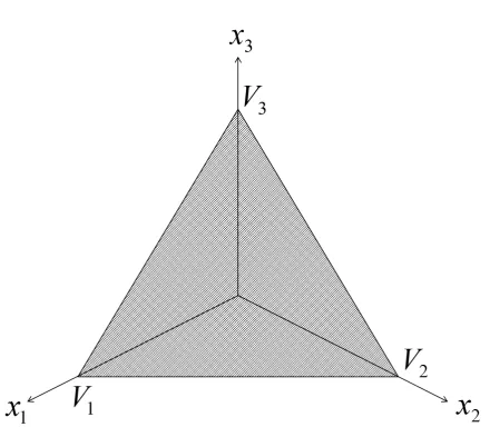
simplex is a triangle, the 3-dimensional simplex is a pyramid, etc. Since the greatest part of

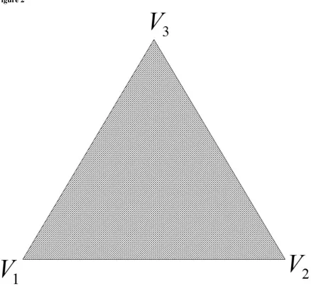
our empirical evidence deals with the 2-dimensional standard simplex (henceforth, standard

2-simplex), we depict it in Figures 1 and 2, where we omit the coordinate axes in Figure 2.

Figure 1. The standard 2-simplex in the Cartesian coordinate system (x1,x2,x3).

- insert Figure 1 here -

Figure 2. The standard 2-simplex (without coordinate axes).

- insert Figure 2 here -

Note that in the Cartesian coordinate system (x1,x2,x3), the vertices of the standard 2-simplex

are given by the coordinates/points

(4) (1,0,0)=:V₁

(5) (0,1,0)=:V₂

(6) (0,0,1)=:V₃

This discussion and Definition 1 imply the following geometrical interpretation of the term

structure: an n-dimensional structure (cf. Definition 1) can be represented by a point on the

(n-1)-dimensional standard simplex. This (n-1)-dimensional simplex contains all the points

that satisfy the definition of the term “n-dimensional structure” (i.e. Definition 1). Two

11

(cf. Definition 1), where X(1),X(2)∈Sn-1, then the structure at t = 2 is not the same as the

structure at t = 1, i.e. structural change took place over the time interval (1,2).

We turn now to a more detailed discussion of the representation of structural change via

functions and trajectories on the standard simplex.

Let us assume the following function:

(7) φ:D×P→S_n−1

(8)

φ

where P is a parameter vector taking values in the set P. (7) and (8) state that the function

) ,

(t P

φ maps time (t) and the parameter vector (P) to the (n-1)-dimensional standard simplex.

In particular, for a given parameter vector P∈P, the function φ(t,P) assigns a point on the

standard simplex (Sn-1), which is located in the coordinate system (x1,x2,…xn), to each time

point t∈D.

Assume an economic model that generates a function φ(t,P) of the type (7)/(8) describing

the structure of the economy ∀t∈D. Since this function assigns a structure to each point in time of the domain D (cf. (3), (7), and Definition 1), we can derive all the information about structural change (cf. Definition 2) in this economic model from this function. In particular,

by studying φ(t,P) we can derive how the structure changes over time for a given setting of

the model parameters P. Therefore, we focus on the analysis of this function, henceforth.

To study the properties of the structural function φ(t,P) geometrically, we use the concept of

trajectory (T(P)), which we define as follows (cf. Definition 1):

(9) ∀P∈P T(P):={φ(t,P)∈Sn₋₁:t∈D}

In fact, T(P) is simply the set of states (or: structures) that the economy experiences (or: goes through) over the time period D for the given parameter setting P. Geometrically speaking, the economy moves along T(P) over the time period D if the parameter setting is P. Note that

definition (9) implies that the structural trajectory T(P) is always located on the standard simplex Sn-1. Thus, we can say that Sn-1 is the domain of the structural trajectory.

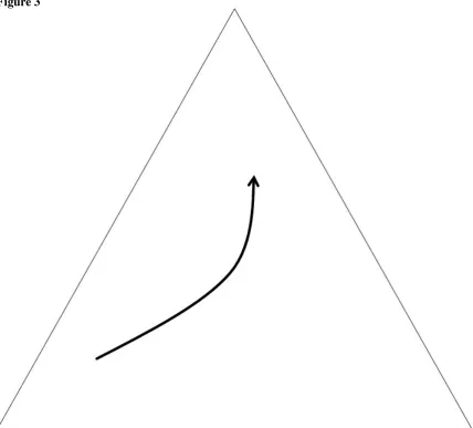
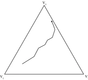
Figure 3 depicts an example of a trajectory given by (7)-(9) and n = 3, where we assume that

) ,

(t P

φ is continuous in t for the given parameter setting P. Note that the arrow in Figure 3

indicates the direction of the movement along the trajectory. Let

φ

the initial point and φ(b,P)≡(x₁b,x₂b,x₃b) be the end-point of the trajectory depicted Figure 3.

Obviously, Figure 3 shows that these points differ. Thus, the trajectory in Figure 3 depicts

12

standard 2-simplex in the Cartesian coordinate system (x1,x2,x3) (cf. Figure 1), we can see

that the trajectory in Figure 3 implies that x₁a >x₁b, x₂a <x₂b and a b x

x₃ < ₃. That is, x1 declined

and x2(x3) inclined over the time period [a,b].

Figure 3. An example of a (continuous) trajectory on the standard 2-simplex.

- insert Figure 3 here -

In general, an economic model and, in particular, a structural change model does not generate

only one trajectory but a family of trajectories, where each family member corresponds to a

different initial state/condition of the economy. This is also a well-known characteristic of

(well-behaving) differential equation systems, where, in general, such a system generates a

family of solutions/trajectories and where each solution/trajectory corresponds to a different

initial condition of the differential equation system. We define such a family of

solutions/functions as follows:

(10) : × → n−₁

I _{D P S}

φ

(11) φI :(t,P): X ≡(x₁,x₂,...x_n)

(12) I∈I

where I is an index (representing the initial condition of the system) taking values in the set I. (10)-(12) state that there is a family of functions indexed by I, where for each index value I∈I

and each parameter setting P∈P, there is a function φI(t,P), which assigns to each time

point t from D a structure φI(t,P) from the simplex Sn-1, which is located in the coordinate

system (x1,x2,…xn). Analogously, we define a family of trajectories by (12) and

(13) ∀I∈I ∀P∈P TI(P):={φI(t,P)∈S_n−1:t∈D}

We can see that for a given parameter vector P, the trajectory TI(P) corresponds to one

function (10) from the family I.

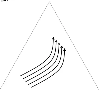
Figure 4 depicts a family of trajectories for n = 3, where we assume that φI(t,P) is

continuous in t for the given parameter vector P and I⊂N.

Figure 4. A family of (continuous) trajectories on the standard 2-simplex.

13

Overall, in this section, we have elaborated all the mathematical concepts that we need to

interpret a structural change model as a family of (parameter dependent) trajectories on the

standard simplex.

3.2 Topological Characterization of (Families of) Trajectories: Continuity and (Self-)Intersection

Trajectories can be characterized by using the concepts of continuity, self-intersection, and in

the case of a family of trajectories, (mutual) intersection. In Sections 5-8, we use these

concepts to characterize the trajectories generated by the theoretical models of the previous

structural change literature and the empirically observable trajectories and to compare theory

with evidence.

The intuitive/geometrical notion of a continuous trajectory is more or less obvious: it is a

curve without interruptions (see, e.g., Figure 3). In contrast, Figure 5 depicts an example of a

non-continuous trajectory.

Figure 5. An example of a non-continuous trajectory on the 2-simplex.

- insert Figure 5 here -

The following definition of a continuous trajectory is obvious.

Definition 3. The trajectory (9) is continuous on Sn-1 (for the parameter setting P), if the

corresponding function φ(t,P) (cf. (7)/(8)) is continuous (in t) on the interval D (for the

parameter setting P). The family of trajectories (13) is continuous on Sn-1 (for the parameter

setting P), if ∀I ∈I, TI(P) is continuous on Sn-1 (for the parameter setting P).

For a definition of a continuous function see some introductory book on analysis.

The geometrical/intuitive meaning of the self-intersection of a trajectory is more or less

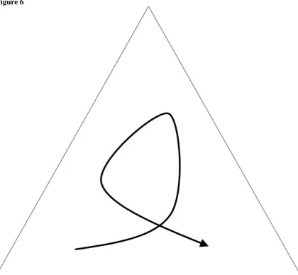
obvious: the trajectory in Figure 3 does not intersect itself, whereas the trajectory in Figure 6

intersects itself.

Figure 6. An example of a self-intersecting (continuous) trajectory on the 2-simplex.

14

We use the following formal definition of non-self-intersection (cf. Stijepic (2015b), p.82).

Definition 4. The (continuous) trajectory (9) is non-self-intersecting (for a given parameter

setting P), if

(14) ∄(t₁,t₂,t₃)∈D3:t₁ <t₂ <t₃ ∧φ(t₁,P)=φ(t₃,P)≠φ(t₂,P)∧P∈P.

Note that per Definition 4, a self-intersection requires that the economy leaves the point

φ

P) at least for some instant of time (t2) before it returns to it (at t3). Thus, according to our

definition, a self-intersection does not occur if the economy reaches some point on Sn-1 (in

finite time) and stays there forever.

A second possibility to define a self-intersecting trajectory is a topological one: a

non-self-intersecting trajectory is homeomorphic to the real line (cf. Section 8.1).

Finally, we define a non-intersecting family of trajectories, as follows.

Definition 5. The (continuous) family of trajectories (12)/(13) is non-intersecting (for the

parameter setting P), if

(15) ∄(G,H)∈I2 :G≠H ∧TG(P)∩TH(P)≠∅∧P∈P.

That is, if we take two different trajectories (G≠H) from the family I, they must not have a point of intersection (i.e., they must not occupy a common point on Sn-1) for a given

parameter setting P. An alternative way to express (15) is: ∀(s,r)∈D2∄(G,H)∈I2 :G≠ H

∧φG(s,P)=φH(r,P)∧P∈P. Figure 7 depicts an intersecting family of trajectories (for a

given P), whereas Figure 4 depicts a non-intersecting family of trajectories (for a given P).

Figure 7. An intersecting family of (continuous) trajectories on the 2-simplex.

- insert Figure 7 here –

3.3 On (Self-)Intersection and Dimension of the Domain of the Trajectory

In this section, we discuss briefly the difference between (self-)intersecting and

non(-self)-intersecting trajectories in relation to the dimension of the space (simplex) in which the

15

characterizing (empirical) trajectories associated with low-dimensional structures (cf.

Definition 1).

We focus here on self-intersections. The same arguments apply to (mutual) intersections.

Imagine a trajectory (T) in the three-dimensional space and assume that the trajectory intersects itself at the coordinate point S (cf. Figure 8).

Figure 8. A self-intersecting (T) and a nearly identical non-self-intersecting trajectory (T’).

- insert Figure 8 here -

It is easy to construct a non-self-intersecting trajectory (T’) that is nearly identical to the trajectory T: we can marginally deform the trajectory T at the coordinate point S such that there is no self-intersection at this point; the trajectory (T’) resulting from this deformation is

nearly identical to the trajectory T (cf. Figure 8). Therefore, it is in some sense “difficult” to distinguish between the self-intersecting trajectory T and the non-self-intersecting trajectory T’. Exactly speaking, whether it is “difficult” or not to distinguish between T and T’ depends

on the mathematical method used. In terms of topology, it is not “difficult” to distinguish

between T and T’: they are not homeomorphic. However, in numerical/quantitative analyses and, in particular, in empirics, where the limits to measurement accuracy and measurement

errors do not allow for a precise determination/construction of trajectories describing

real-world processes, the “difficulties” are significant. In general, it is not possible to determine

whether the process measured by the data generates a(n) (self-)intersection. For example, if

our data implies that there is a(n) (self-)intersection, we could argue that there would not be

a(n) (self-)intersection, if we increased the accuracy of measurement (i.e. the number of digits

after the decimal point).

In contrast, (self-)intersection of trajectories in two or one-dimensional space is easier to

detect. In general, trajectories (of significant length) partition the two-dimensional space

significantly, such that a(n) (self-)intersection is easy to detect (cf. Stijepic (2015b), p.82f).

This fact becomes obvious in Section 6 where we identify (self-)intersection of empirical

trajectories on two-dimensional simplexes.

4. ON STRUCTURAL CHANGE MODELS AND THEIR TRAJECTORIES AS EXPLANATIONS OF EMPIRICAL OBSERVATIONS

In this section, we discuss how the structural dynamics of a country or a group of countries

16

change models. This discussion does neither refer to a specific empirically observed

characteristic of structural change trajectories nor does it discuss a specific structural change

model from the previous literature, but is rather of methodological character: while it is quite

straight forward how to explain the dynamics of one country by using a structural change

model (cf. Section 4.1), there are different ways (or approaches) to explain the dynamics of a

group of countries by using a structural change model (cf. Section 4.2); as we will see in

Section 4.2.4, these ways reflect different (methodological) views on the notion of economic

law underlying the structural change models. In Section 5, we use these (methodological)

results to develop approaches for explaining a specific sort of empirical evidence, namely the

(self-)intersection of trajectories.

4.1 Explanation of a Country’s Dynamics

Assume that we have data on the dynamics of a structure (e.g. dynamics of labor allocation)

over some period of time (e.g. 1820-2003) in a country (e.g. the US). Furthermore, assume

that we construct this country’s structural trajectory on the simplex by using this data (cf.

Section 6). Figure 9 depicts an example of such a trajectory.

Figure 9. Trajectory of labor allocation across agriculture, manufacturing, and services in

the US between 1820 and 2003.

- insert Figure 9 here –

Notes: Data source: Maddison (2007). See Section 6.2 for method description.

Assume now that we would like to have a theoretical explanation of the dynamics depicted

by the trajectory (in Figure 9). To do so, we can choose an existing structural change model

(e.g. the Kongsamut et al. (2001) model) and analyze first, whether the model can explain

(certain characteristics of) the observed trajectory. This can be done as follows. First, solve

the model equations and obtain in this way a family of functions of the type (10)-(12). Note

that for a given parameter vector P, (10)-(12) imply a family of trajectories corresponding to

different initial values of the system/economy; cf. (13). Thus, among the family members (I), we must choose the trajectory that goes through the empirically observed initial state6 of the

(US) economy. Second, choose the model parameters (P) such that the model trajectory

6

17

corresponding to the observed initial state of the country is as similar7 as possible to the

empirically observed trajectory of the country. The term “similar” may here refer to

qualitative aspects, e.g. the shape and orientation of the trajectory on the simplex, or

quantitative aspects, where the latter refer to the question whether the model generates

changes in the structure that are of similar (numerical) magnitude as the changes observed in

reality for the given initial value of the country considered.

That is, to analyze whether the model can explain (certain characteristics of) the empirically

observed structural trajectory of a country, we compare the (most suitable) trajectory

generated by the model and the empirically observed trajectory of the country. If the model

trajectory is sufficiently similar to the observed trajectory we can say (under many

restrictions) that the model is a theoretical explanation of the country’s dynamics.

4.2 Explanation of the Dynamics of a Group of Countries and Relation to Economic Laws

In this section, we discuss how observable cross-country differences regarding the qualitative

(and quantitative) properties of the structural trajectories can be modelled by using a

structural change model. In particular, the validity of the statements made in this section is

not restricted to (only) one of the specific standard structural change models (discussed in

Section 2.2), but has rather general character, since we rely again on the mathematical

meta-model (10)-(13), which covers a wide range of specific structural change meta-models. Examples

of specific structural change models are discussed in Sections 2.2, 7, and 8.1. Furthermore, in

Section 4.2.4 we discuss the implied methodological view of models as representing laws.

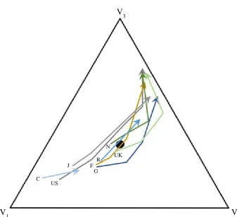
Now, assume that we depict the empirically observed trajectories of different countries (e.g.

OECD countries) on one and the same simplex (see, e.g., Figure 10) and aim to provide a

joint explanation for the dynamics of these countries by using a structural change model (e.g.

the Kongsamut et al. (2001) model). Since the empirically observed structural dynamics and,

thus, the trajectories of the countries differ significantly (as shown, e.g., in Section 6), we

cannot explain the dynamics of all countries by only one model trajectory. That is, we need a

model that generates multiple trajectories that differ from each other.

The meta-model (10)-(13) implies three approaches of generating multiple/different

trajectories in a model. (We use these approaches later in Section 5.2.)

7

18 4.2.1 Approach 1

As implied by (13), the dynamic system (10)-(12) generates a family (of different)

trajectories for a given parameter setting (P), where each trajectory corresponds to a different

initial value of the system. Thus, to model cross-country heterogeneity regarding trajectories,

we can assume that (a) all the countries have the same parameter values, i.e. the parameter

vector (P) does not differ across countries, and (b) the countries differ by initial conditions. In

this case, the countries belong to the same family (I) of trajectories, where each I∈I represents a country and, in particular, a different initial condition. Example 9 may elucidate

these explanations.

Example 9 (Approach 1). Assume that we aim to explain the dynamics of US, UK, and

Japan by using a model that generates a trajectory family of the type (10)-(13). It is possible

to assign (qualitatively and quantitatively) different trajectories of this model to the different

countries, if we assume that the dynamics of US, UK, and Japan can be described by

(10)/(11)/(13) and choose the function φA(t,P) for US, φB(t,P) for UK, and φC(t,P) for

Japan, where P∈P, A,B,C∈I and A≠B≠C≠A. As we can see, the index I differs across countries, whereas P is the same for all countries.

We apply Approach 1 in Section 5.2 to derive a method for generating trajectory intersections

in standard structural change models via parameter perturbations.

4.2.2 Approach 2

As implied by (13), cross-country differences in (qualitative and quantitative) trajectory

characteristics can arise if we assume that parameter values (P) differ across countries. In this

case, cross-country differences in initial conditions are not necessary to create heterogeneous

trajectories within a model (although due to empirical evidence, it may be reasonable to

assume that cross-country differences in initial conditions exist). In other words, Approach 2

assumes that all countries have the same index I (cf. (12)), but differ in parameters P.

Example 10 elucidates Approach 2. The discussion in Section 5.2 implies that Approach 2 is

useful for explaining the structural change evidence when relying on standard structural

19

Example 10 (Approach 2). Assume that we aim to explain the dynamics of US, UK, and

Japan by using a model that generates the trajectory family (10)-(13). It is possible to assign

(qualitatively and quantitatively) different trajectories of this model to the different countries,

if we assume that the dynamics of US, UK, and Japan can be described by (10)/(11)/(13) and

choose the function φI(t,A)

for US, φI(t,B)

for UK, and φI(t,C)

for Japan, where I∈I,

A,B,C∈P and A≠B≠C≠A. As we can see, the parameter values (A,B,C) differ across countries, whereas the index I is the same for all countries.

4.2.3 Approach 3

Approaches 1 and 2 refer to the explanation of structural change in different countries by

using only one structural change model, e.g. the Kongsamut et al. (2001) model. A third

approach could be developed by going beyond initial condition differences (Approach 1) and

parameter differences (Approach 2) and assuming that each country follows its own model.

This may make sense when the structural change determinants differ strongly across

countries such that, e.g., US structural change is best described/explained by the Kongsamut

et al. (2001) model and UK structural change is best described/explained by the Ngai and

Pissarides (2007) model. We can express such model differences by using the mathematical

formalism introduced in Section 3.1 as follows. By referring to our US-UK example, assume

that US structural change is described by the system (10)-(12) and UK structural change is

described by the system

(10’) : × → n−₁

J _{D Q S}

ϕ

(11’) :(, ) ( 1, 2,... n)

J x x x X Q

t : ≡

ϕ

(12’) Q∈Q

That is, the UK and US systems follow different functional forms (

φ

ϕ

different parameter vector spaces (P vs Q).

Three aspects of Approach 3 are noteworthy.

First, very strong differences in economic assumptions can be represented as differences in

model parameters (Approach 2). Recall that the changes in only one parameter value (e.g. the

elasticity of substitution) in economic models can cause very strong changes in economic

assumptions (e.g. Leontief-type vs. Cobb-Douglas-type utility/production function).

Second, in many cases, it is possible to generate meta-models that cover many different

models as parameter special cases. That is, in many cases, Approach 2 covers Approach 3.

20

transform into the Kongsamut et al. (2001) model or the Ngai and Pissarides (2007) model

under certain parameter constellations. That is, the latter models are special cases of the

former models that arise for certain parameter values (P). This example proves that it is

possible to cover the cases belonging to Approach 3 by Approach 2 (and 1).

Third, Approach 3 implies/presumes that the structural change models represent “ad hoc

laws”, which may be a point of critique for methodological reasons, as discussed in Section

4.2.4.

4.2.4 The relation between the three approaches and the types of economic law

The general notion of “a law” as used in natural sciences (and economics) refers to a

regularity that is valid/persistent across time and space. If we use this notion in economics,

we would refer to a (general) economic law as a regularity that is persistent across time and

countries. Thus, this regularity can be used for predicting future dynamics in different

countries. More generally speaking, the existence of some sort of economic law is the basis

for any prediction of economic dynamics. For a discussion of laws in economics and natural

sciences, see, e.g., Jackson and Smith (2005) and Reutlinger et al. (2015).

Our discussion of Approaches 1-3 is closely related to the methodological discussion of the

economic models regarding the economic laws they represent.

Approach 1, assuming that one and the same model and one and the same parameter vector

can explain structural change in all time periods (considered) and in all countries,

corresponds to the general notion of a (natural) law, i.e. a regularity that is valid/persistent

across time (“all periods”) and space (“all countries”).

In contrast, Approach 2 assumes that empirical observations can be explained by one and the

same model, only if we allow that parameters vary across countries. Thus, Approach 2

corresponds to the view that economic models represent “ceteris paribus laws”. The latter are

widespread in economic modeling. See Reutlinger et al. (2015) for a discussion.

Approach 3 corresponds to “ad hoc laws”, i.e. regularities that are sometimes applicable and

sometimes not. In particular, the applicability of an ad hoc “law” differs from country to

country, while (in contrast to ceteris paribus laws) it is not clearly stated when the model is

applicable and when not. From the methodological point of view, the models representing

21

are directly testable by empirical evidence, in contrast to ad hoc models.8 Furthermore, in

structural change modeling, “ad hoc laws/models” seem unnecessary, since there are many

similarities in structural change patterns across countries, which can be modeled as (ceteris

paribus) laws. In particular, it is, therefore, possible to replace “ad hoc laws” by “ceteris

paribus laws”, where the latter can account for cross-country differences in structural change

patterns, while being testable and explicitly naming the parameters that are responsible for

the observable differences across countries.

For these reasons, Approaches 1 and 2 (“general law” and “ceteris paribus law”) seem to be

preferable over Approach 3 (cf. Section 5.2).

5. ON DIFFERENT WAYS OF GENERATING (SELF-)INTERSECTING TRAJECTORIES IN MODELS DESCRIBED BY DIFFERENTIAL EQUATIONS

While Section 4 discusses the general/methodological aspects of the theoretical explanation

of trajectory-related empirical evidence, Section 5 is more specific and discusses how a

specific type of trajectory-related empirical evidence, namely the (self-)intersection of

trajectories, can be explained by structural change models that are described by differential

equation systems. Especially, Section 5.2.1 merges the (methodological) results from Section

4 with some lessons from the mathematical theory of differential equations to derive concrete

approaches for generating intersecting trajectories in (structural change) models that are

described by differential equation systems. Note that the focus on differential equation

systems (as opposed to general dynamical systems) in this section is justified by three facts:

(a) the most structural change models are representable by differential equations, since the

typical long-run modeling assumptions rely on smooth (production and utility) functions; for

example, all the models discussed in Section 8 are continuous and differentiable (with respect

to time); (b) the most economists are familiar with the basic aspects of differential equations;

and (c) we can rely on the many useful results of the mathematical literature on differential

equations. In contrast, in Section 8, we do not rely on differential equations as descriptions of

structural change but on a more topological approach based on homeomorphisms.

We start the discussion in Section 5.1 by recapitulating the well-known result from

differential equation theory that smooth autonomous differential equation systems generate

only non-(self-)intersecting trajectories for given/constant system parameters. Then, we

discuss how deviations from this standard case can generate intersecting (cf. Section 5.2.1)

8

22

and self-intersecting (cf. Section 5.2.2) trajectories. In each section, we discuss as well which

of these deviations can be used for generating (self-)intersections in Section 7.

5.1 Autonomous Differential Equation Systems and Non-(Self-)Intersection

In this section, we recapitulate some standard differential equation theory, which is the basis

for our discussion (e.g. in Section 5.2). For references on all the statements, see, e.g., Stijepic

(2015b), p.84f.

Assume a model (cf. Section 7) that generates the following initial value problem associated

with an autonomous n-dimensional differential equation system:

(16) ∀t∈D'⊆R ∀X₀ ∈U'⊆Rn ∀P∈P' dX(t)/dt =Φ(X(t),P), X(0)= X₀, 0∈D'

where P is a parameter vector taking values in the set P’. It is well known from the mathematical literature on differential equations that there exists a unique solution of (16) (on

a set U⊆U’, a set P⊆P’, and an open interval D⊆D’ containing 0) if the function Φ has

certain (smoothness) characteristics9 (for P

∈

family of functions φI : D×P→U (with the index I∈I and the parameter vector P∈P) that

has the following characteristics: (a) the corresponding family of trajectories (TI(P):= {φI(t,

P)∈U: t∈D}, where I∈I and P∈P) is continuous and non-intersecting (cf. Definitions 3 and

5), and (b) ∀P∈P, ∀I∈I, TI(P) is non-self-intersecting (cf. Definition 4).

Overall, a unique solution of (16) generates a family of trajectories that are continuous,

non-intersecting, and non-self-intersecting (cf. Definitions 3-5) for a given parameter setting (P).

In other words, if the structural dynamics are representable by a model of smooth

autonomous differential equations with a given parameter vector, (self-)intersections do not

arise (cf. Approach 1, Section 4.2.1). Therefore, we discuss now how to generate

(self-)intersections by deviating from this model.

5.2 Some Mathematical Models of (Self-)Intersection

In this section, we present several mathematical conditions under which self-intersection of a

(country’s structural) trajectory and intersection of the members of a family of trajectories

(where each trajectory belonging to the family represents the structural dynamics of a

country) can occur. The discussion is based on the standard results of the mathematical

9

23

literature on differential equation systems. To demonstrate the applicability of the results of

Section 5.2, we apply them in Section 7 for analyzing under which conditions can the

Kongsamut et al. (2001) model generate (self-)intersecting trajectories.

5.2.1 Models of families of intersecting trajectories

Assume that we observe structural change in two countries. For each of the two countries, we

construct a structural trajectory based on the empirical data. Furthermore, assume that the two

trajectories intersect. (We will see in Section 6 that this is a common empirical observation.)

We discuss now how this intersection can be modelled or explained by using the concepts

introduced in Sections 4.2 and 5.1.

Intersections between two trajectories representing two different countries (country A and

country B) can occur in the following five cases, which are implied by the standard

mathematical theory of differential equation systems.

a) Non-autonomous differential equation systems (time-varying “law”). Assume that the

structural changes in the two countries under consideration follow one and the same

structural “(pseudo) law” and that the latter can be expressed as follows

(17) ∀t∈D⊆R ∀X₀∈U⊆Rn dX(t)/dt=Γ(X(t),t), X(0)=X₀, 0∈D

Furthermore, assume that country A has the initial condition X(0) = A∈U and country B has the initial condition X(0) = B∈U, where A≠B. Implicitly, we assume here that both countries have the same parameter vector; therefore, (17) does not display the parameter

vector explicitly. All these assumptions imply that we rely here on Approach 1 (cf. Section

4.2.1). We can see that Γ is not only dependent on X but also on time and, thus, the

differential equation system (17) is autonomous. It is well known that the

non-autonomous differential equation system (17) can generate trajectories that intersect each

other (cf. Definition 5) even if Γ is smooth in the sense discussed in Section 5.1. Thus, the

“(pseudo) law” (17) may imply that the trajectories (of the two countries following this law

and having different initial conditions) intersect in the sense of Definition 5.10 We do not use

10

non-24

this approach (i.e. non-autonomous systems) in Section 7, since the model discussed there

can be represented by an autonomous differential equation system.

b) Non-smooth vector fields. Following Approach 1 (cf. Section 4.2.1), assume that: (i) the

structural law (followed by the two countries) is described by the autonomous differential

equation system (16); (ii) both countries have the same parameter values (P); (iii) the two

countries have not the same initial conditions; and (iv) Φ does not satisfy the usual

smoothness conditions discussed in Section 5.1, such that the solution of (16) is not unique in

the sense used in Section 5.1. Such a solution can be associated with a family of intersecting

trajectories. Thus, the trajectories of the two countries modelled by this system could

intersect each other (if the initial conditions of the countries are not the same). As noted at the

beginning of Section 5, the typical structural change models (and most of the long-run growth

models) are continuous and assume smooth (utility and production) functions such that the

resulting dynamical systems are smooth. Therefore, among others, we cannot rely on

non-smooth vector fields as an explanation of intersection in Section 7.

c) “Law” differs across countries. Following Approach 3 (cf. Section 4.2.3), assume that the

structural “(pseudo) law” in country A can be described by (16) (with a fixed parameter

setting P), and the structural “(pseudo) law” in country B can be described by

(18) ∀t∈D⊆R ∀X₀∈U⊆Rn dX(t)/dt=D(X(t)), X(0)=X₀, 0∈D

Furthermore, assume that Φ and D are sufficiently smooth such that unique solutions of

(16) and (18) exist (and, thus, each system generates a family of continuous and

non-intersecting trajectories (cf. Definition 5)). These assumptions state that each country follows

its own “(pseudo) law” (i.e. the “laws” are ad hoc); thus, the trajectories of the countries

could intersect despite the existence of unique solutions for each country. As discussed in

Section 4.2.4, ad hoc models are not only inferior to the models that generate statements that

are valid across several countries but also can be replaced by “ceteris paribus models/laws”

(see point d) when modelling structural change.

25

d) Ceteris paribus laws.Assume that the structural law can be expressed by (16), where P is a

parameter vector taking values in the set P⊆P’. Furthermore, assume that Φ is sufficiently

smooth such that there exists a unique solution of (16) (for each P∈P) corresponding to a family of non-intersecting trajectories. Let the two countries under consideration follow the

law (16) and differ only by P, i.e. country A has the parameter value P = A∈P and country B

has the parameter value P = B∈P, where A≠B. We can see immediately that these

assumptions reflect Approach 2 (see Section 4.2.2) and that the law (16) is a ceteris paribus

law (see Section 4.2.4). In this case, cross-country differences regarding the trajectory

characteristics are generated by cross-country parameter variation.

e) Parameter perturbations. Assume that the two countries follow the law (16) and that Φ is

sufficiently smooth such that there exists a unique solution of (16) (for each P∈P⊆P’ and for

all X(0)

∈

assume that both countries are characterized by the same P (i.e. country A has the parameter

value P = C∈P and country B has the parameter value P = C) but differ by initial conditions (i.e. country A has the initial condition X(0) = A

∈

∈

assume that one country is a latecomer (i.e. moves slowly through the state space) and

intersects after the perturbation the pre-perturbation segment of the fast-developing country.

This can occur even in structurally stable systems, since structural stability does not prevent

intersection of the perturbed and non-perturbed system. This effect can occur easily in

systems with bifurcations. Finally, note that case e reflects Approach 1 (cf. Section 4.2.1)

with parameter perturbations.

Note that the cases a to e are archetypes. It is possible to create intersections by combining

these archetypes. For example, we could generate intersections by assuming that the two

countries follow one and the same ceteris paribus law (case d) and are subject to

(asymmetric) parameter perturbations (case e).

Overall, the discussion of the points a to e shows that we will rely on cross-country parameter

differences (case d) and parameter perturbations (case e) (or some combination of them)

26 5.2.2 Models of self-intersecting trajectories

Now, we turn to the question under which circumstances a self-intersection of a trajectory

(representing the structural dynamics of a country) can occur, where, again, we use the

concepts described in Section 5.1 to answer this question. A self-intersection of a country’s

structural trajectory can occur in the following cases.

i) Non-autonomous differential equation systems (time-varying “law”). Assume that the

country follows the law implied by the non-autonomous differential equation system (17) and

that the initial state of the country is given, i.e. X(0) = X0∈U. It is well known that the

solution of non-autonomous systems of type (17) for a given initial value can be associated

with self-intersecting trajectories in the sense of Definition 3.

ii) Non-smooth vector fields. Assume that (I) the structural law (followed by the country) is

described by the autonomous differential equation system (16), (II) the parameter vector (P)

is fixed, and (III) Φ does not satisfy the usual smoothness conditions discussed in Section

5.1, such that the solution of (16) is not unique in the sense used in Section 5.1. For a given

initial condition X(0) (representing the country’s initial state), such a solution could be

associated with a self-intersecting trajectory (describing the dynamics of the economy).

iii) Parameter perturbations. Assume that: (I) the country follows the law (16); (II) Φ is

sufficiently smooth such that there exists a unique solution of (16) (for each P∈P⊆P’ and for

all X(0)

∈

state of the economy is given, i.e. X(0) = X0∈U; and (IV) initially, the parameter value for

the country is given by P = C∈P. Assume now that a perturbation of P occurs at some point in time t = z > 0, i.e. P = C for t < z and P = C’∈P for t ≥ z, where C≠C’. In this case, the post-perturbation (t > z) segment of the country’s trajectory can intersect the pre-perturbation

(t < z) segment of the country’s trajectory, such that the overall trajectory (which is the union

of the post- and pre-perturbation segment) intersects itself according to Definition 3. This can

occur even in structurally stable systems, since structural stability does not prevent

intersection of the perturbed and non-perturbed system.

For the reasons discussed in Section 5.2.1 (points a and b), we can exclude alternatives (i)

self-27

intersections by assuming that there are perturbations of the parameters (case iii) of the

Kongsamut et al. (2001) model.

6. EVIDENCE ON THE TOPOLOGICAL PROPERTIES OF STRUCTURAL CHANGE TRAJECTORIES AND STYLIZED FACTS

Sections 6-7 can be regarded as an application of the method developed in Sections 2-5 to

different topics covered by our definition of structural change. Since our definition of

structural change (i.e. Definition 2) and method (i.e. topological approach) cover a wide

range of topics (cf. Section 2.2), it is not possible to discuss the evidence on

(self-)intersection of trajectories associated with all these topics. Therefore, in Section 6.2, we

focus on a specific type of structural change covered by Definition 2, namely, labor

re-allocation across agriculture, manufacturing, and services. Nevertheless, in Section 6.1, we

discuss briefly evidence on (non-)self-intersection of trajectories associated with some other

topics covered by Definition 2, since it is relatively easy to construct this evidence on the

basis of well-known and well-available data.

6.1 On the Construction of Evidence on Non-Self-Intersection of Trajectories Associated with Definition 2

Following Stijepic (2015b), p.82f, it can be relatively easy to identify non-self-intersection in

empirical data on structural change. Assume that we have data on the vector X(t)≡

(x1(t),x2(t),…xn(t)) for the time points t0, t1, t2,…tm. The corresponding trajectory T:= {X(t) : t

∈

∈

with the property that xi(t) increases or decreases monotonously over the period t0, t1, t2,…tm.

By using this proposition, we can easily identify non-self-intersecting trajectories by relying

on well-known data, as demonstrated in Examples 11 and 12.

Example 11. Kongsamut et al. (2001), p.873, provide data on the US consumption structure

(cf. Example 8) in the three-sector framework (cf. Example 2). The data depicts the dynamics

of the agricultural, manufacturing, and services consumption shares over the period

1940-2000. As this data reveals, besides some short-run fluctuations, the consumption share of

services increases monotonously over this period. Thus, we can conclude that the trajectory

representing the Kongsamut et al. (2001) data on the consumption structure in the