Space time patterns of rank concordance: Local indicators of mobility association with application to spatial income inequality dynamics

Munich Personal RePEc Archive

Space-time patterns of rank concordance:

Local indicators of mobility association

with application to spatial income

inequality dynamics

Rey, Sergio

Arizona State University

11 February 2016

Online at

https://mpra.ub.uni-muenchen.de/69480/

Space-Time Patterns of Rank

Concordance: Local Indicators of

Mobility Association with Application

to Spatial Income Inequality

Dynamics

1 2

S

ergio

J. R

ey

GeoDa Center for Geospatial Analysis and Computation

School of Geographical Sciences and Urban Planning

Arizona State University

[email protected]

1_{This is an Accepted Manuscript of an article published by Taylor & Francis Group in: Annals of the}

Association of American Geographers. DOI: 10.1080/24694452.2016.1151336.

2_{Code and data to reproduce the results of this article are available athttp://github.com/sjsrey/}

limaaag.

Abstract

1. I

ntroduction

Disparities in the levels of income between individuals in a society have long attracted attention

across a variety of disciplines and have now assumed center stage in both policy and scientific

circles (Stiglitz, 2012; Piketty, 2014). This attention reflects the concern that inequality can have

negative impacts on social welfare and cohesion, as well as on economic growth (Cramer, 2003;

Partridge, 1997).

Inequality at one point in time represents a snapshot of the path of the income distribution’s

evolution. That snapshot characterizes the outcomes of socioeconomic processes. While large

inequalities in these outcomes draw much concern, it is important to keep in mind that the

snapshot distribution is static and ignores any dynamics at work in the distribution’s evolution.

One response to this shortcoming has been the rise of the distribution dynamics literature (Quah,

1996b; Maasoumi et al., 2007) that adds a dynamic lens to the question of inequality. Here,

measures of the external properties of the distribution, which include inequality indices, are

tracked over time to provide a more comprehensive view of inequality dynamics.

The focus on the external properties of the distribution misses what some have argued is an

equally important concept to inequality, and that is economic mobility (Fields, 2010; Hammond

and Thompson, 2006; Schorrocks, 1978). Consider two societies with equally high levels of

inequality and similar external distribution dynamics such that dispersion in the distribution

is increasing over time. From this perspective the two systems would seem indistinguishable

regarding their respective inequality dynamics. Yet the welfare of individuals from each of these

societies would be different if one of the systems displayed higher income mobility than the other,

since the opportunities for changing one’s position in the distribution would be improved.

Economic mobility is, however, less clearly defined than economic inequality as a number of

different types of mobility have been described. One distinction is between absolute and relative

mobility. When individuals move away from their initial levels of income in a distribution absolute

mobility occurs. Relative mobility is more of a re-ranking phenomena whereby the movement of

an observation in the distribution is considered with respect to the positions of other observations

in the distribution (Formby et al., 2004). In other words, relative mobility occurs when the ordinal

positions change over time, whereas absolute mobility reflects changes in the cardinal positions.

(Maasoumi, 1998).

The income inequality literature has preceded the mobility literature in identifying the need

for, and incorporating, a spatial perspective. This reflects the recognition that income disparities

between countries are the focus of the literature despite often being smaller than disparities within

countries (The Economist, 2011). From a policy perspective, regional disparities have motivated

for the establishment of programs targeting economic development (Jalan and Ravallion, 1998;

Bigman and Srinivasan, 2002). A related question is how intergenerational income mobility may

vary depending upon geographical context (Chetty et al., 2014). On the methodological front the

dominant theme is work on spatial inequality decomposition where economies within a national

system are placed into mutually exclusive and exhaustive regions and then overall inequality is

decomposed into that due to disparities between economies from different regions and that due

to disparities among economies within each of the regions. A common finding across the large

corpus of these studies is that within region inequality tends to dominate inequality between

regions (Shorrocks and Wan, 2005, p. 68).

While the inequality literature has taken the spatial turn sooner than the mobility literature

has, there have been some recent extensions of distributional dynamic approaches that incorporate

spatial considerations. Discrete Markov chains (Quah, 1996a; Magrini, 1999) and rank correlation

statistics (Webber et al., 2005; Cuadrado-Roura, 2009) have played a central role in this regard.

The discrete Markov chain framework has been enhanced to allow for regional conditioning of

the transitional probabilities using so-called spatial Markov chains (Rey, 2001; Le Gallo, 2004). A

second extension has been the development of a space-time version of a rank correlation measure

of income mobility (Rey, 2004). Spatio-temporal rank correlation examines the extent to which the

overall mobility, or changes in the ranks of economies, displays a geographical pattern or not.

These spatial extensions to mobility measures are required to assess the extent to which

spatial dependence and/or spatial heterogeneity are present. Non-spatial approaches to inference

regarding income mobility indices are based on the assumption of independence (Schluter, 1998;

Formby et al., 2004), and thus their use in a spatial context is problematic. At the same time,

existing spatial mobility measures are global in nature. That is, they report on the extent of spatial

dynamics in the sense that the movements of an individual region in the income distribution over

time are related to those of its neighboring regions.

In this article I extend Rey (2004) to develop a family of local indicators for mobility analysis

(LIMA). These allow for a decomposition of the global measure of spatial rank concordance into

spatially explicit contributions associated with each individual regional observation. Different

forms of the LIMA are suggested that allow for alternative representations of regional context. As

a complement to the local measures, I also suggest that the additive nature of the decomposition

of the LIMAs permits the development of meso-scale measures of interregional mobility that

can be used to examine the distinction between interregional and intraregional income mobility

dynamics, analogous to the approach used in the interregional inequality literature (Kanbur and

Venables, 2005). I also propose approaches to inference for the LIMAs and their interregional

decomposition.1

In the remainder of the article I first revisit the global indicator of spatial concordance that

serves as the foundation for the derivation of the local measures (Section 2). Next a family of

local indicators for mobility analysis are presented along with a meso-scale level indicator that

considers the concepts of interregional and intraregional distributional mobility (Section 3). These

measures are examined in an empirical application of Mexican state per capita gross domestic

product dynamics over the period 1940-2000 (Section 4). I close the article with some concluding

comments and the identification of future research directions (Section 5).

2. G

lobal

I

ndicators of

M

obility

A

ssociation

The departure point for the development of spatial measures of mobility is the general rank

correlation coefficient originally suggested by Kendall (1962):

τ(g,f) = ∑

n−2

i=0 ∑

n−1

j=i+1sgn(fi−fj)sgn(gi−gj)

n(n−1)/2 =

c−d

n(n−1)/2 (1)

where f andgare variables with observations overi=1, 2, . . . ,nunits. The numerator reflects the

net-concordance between all pairs of observations on these two variables, wherecis the number

1_{The focus in this paper is on new methods for the analysis of regional income inequality dynamics. The literatures on}

of concordant pairs, andd the number of discordant pairs. As a correlation measure the range

is−1≤τ(g,f)≤1. For small samples the exact distribution ofτ(g,f)can be obtained through

full enumeration under the null of rank independence. Asymptotically τ(g,f) has a normal

distribution with mean 0 and variance ₉4_nn_(n+₊10₁₎.

In the convergence literature the two variables are defined as incomes in an initial (fi=yi,t0)

and ending period (gi =yi,t1), respectively. Given the range ofτ(g,f)the sign of the coefficient

matters when considering mobility or rank changes in the distribution. Thus a derived measure of

mobility could be defined as:

M= τ(g,f)−1

−2 (2)

with 0 ≤ M ≤ 1. Economies with larger values of M would display greater distributional

mixing over a given period relative to those economies with lower values ofM. Note that having

τ(g,f) =0 does not imply the absence of rank mobility, rather a value ofτ(g,f) =1 would.

2.1. Spatial Decomposition of Rank Mobility

In Rey (2004) a spatial version of Kendall’s statistic was based on a decomposition of the pairs into

those that are geographical neighbors and those that are not. Define the matrixSwith elements

si,j =1 if observationsi,j are concordant,si,j =−1 ifi,jare discordant, andsi,j =0 otherwise,

then equation (1) can be redefined using:

c−d= 1

2

∑

∑

to give:

τ(g,f) = ι′Sι

n(n−1) (3)

withιthe(n×1)unit vector. LetW denote a binary spatial weights matrix with elementswi,j=1

if observationsiandjare geographical neighbors, 0 otherwise, and ¯W =ιι′−W−I, we can then

define the matrixS:

S=W◦S+W¯ ◦S (4)

Noting thatι′(W+_W¯_{)ι=n(n−1)we have:}

τ(g,f) = ι

′_{(W◦S+W¯ ◦S)ι} ι′(W+W¯)ι =

ι′(W◦S)ι+ι′(W¯ ◦S)ι

ι′(W+W¯)ι (5)

or, equivalently:

τ(g,f) = ι

′_Wι ι′(W+_W¯_)ι

ι′(W◦S)ι ι′Wι +

ι′W¯ι ι′(W+_W¯_)ι

ι′(W¯ ◦S)ι

ι′W¯ι =ψτw(g,f) + (1−ψ)τw¯(g,f) (6)

which has the classic rank correlation statistic as a weighted average of the rank correlation for

neighboring pairs and that for the non-neighbor pairs withψ= ι′Wι ι′(W+W¯)ι.

The decomposition determines whether the classic measure masks different correlation patterns

between the two pair sets: neighboring and non-neighboring. Inference on this question can be

based on random spatial permutations of the attributes to develop a distribution forτwunder the

null of spatial homogeneity in the correlation patterns between the neighbor and non-neighbor

pairs. As this statistic yields a single value for the amount of rank mobility in the entire distribution

over two points in time it can be considered aGlobal Indicator of Mobility Association(GIMA). Given

the relationship between the traditionalτfrom (1) and the derived mobility index in (2), a spatial

mobility measure can be defined as:

MW=

τW−1

−2 . (7)

This also allows for an additive decomposition of overall mobility:

M=ψMW+ (1−ψ)M_W¯. (8)

To illustrate this GIMA consider Figure 1 which displays the spatial distribution of ranks on a

map of 16 regularly sized regional units at periodt0(Figure 1a) and periodt1(Figure 1b). Also

shown is a partition of the units into four regimes (Figure 1c) which can be used to operationalize

neighbors using so called block weights (Anselin and Rey, 2014, p. 37) such thatWi,j = 1 if

R(i) =R(j), otherwiseWi,j=0, whereRis a function that maps an observation to its regime.

[Figure 1 about here.]

(i.e., 16*15/2) pairs, 114 are concordant over the two periods, while 6 pairs are discordant. Close

inspection of the rank distribution in the second period reveals that the 6 discordant pairs are

contained in regime 3. The spatially focused nature of the discordance is reflected in the lower

rank correlation value for the neighbors,τW=0.50. Moreover, all of the non-neighbor pairs are

concordant givenτW¯ =1.00. Based on 999 random permutations, the spatialτwis significant at

p=0.001 indicating different concordance relationships are found between the neighboring and

non-neighboring pairs.

A second example can be seen in Figure 2. Here the rank distribution in the first period is the

same as the previous case but the rank distribution has changed in a different fashion (Figure 2b).

Members of regime 1 leapfrog those in regime 0, and those in regime 2 now swap ranks with

those in regime 3. As a result, the overall rank correlation dropsτ=0.467, however the spatial

rank correlation measure is at τW = 1.0 as the ordinal relations for all neighbor pairs remain

constant over the two periods. Based on 999 random spatial permutations of the observations on

both variables jointly, the p-value for theτW is 0.002. Because the same spatial permutation is

applied to both time periods, the overall amount of mobility will be maintained across each of the

permutations.

[Figure 2 about here.]

2.2. Space-Time Concordances and Spatial Autocorrelation

When cross-sectional observations are available over multiple time periods, a common analytical

strategy is to apply a global measure of spatial autocorrelation to explore how spatial dependence

may be evolving overtime (Rey and Montouri, 1999, p. 146). It is important to note that space-time

concordance, as measured using the spatial τW above, focuses on different properties of the

changes in a spatial distribution from those offered by existing global spatial autocorrelation

measures applied in a space-time context. Returning to the example in Figure 1, the application of

Moran’s I using the regime weights yields identical values for the global spatial autocorrelation

statistic in both periods, despite the change in the spatial distribution. By contrast, we see that

the classicτ(0.90) and the spatialτW(0.50) now reflect lower concordance between the spatially

level of spatial autocorrelation declines slightly in the second period (0.775 vs. 0.740) whereas the

global classicτremains at 0.90 and the spatialτW is now 0.667. While the latter has increased

in value relative to the case when the block weights were used, it remains statistically significant

pointing to different concordance relations for the neighboring and non-neighboring pairs.

These two examples illustrate that space-time concordance and changes in spatial

autocorrela-tion over time are not identical. The space-time concordance measures consider how the pairwise

ordinal associations between neighboring values evolve over time, while the difference in the

global autocorrelation statistic captures how pairwise interval associations change between time

periods. The two measures should be thought of as complements and not substitutes because they

capture different aspects of spatial distribution dynamics. This will be explored more fully below.

3. A F

amily of

L

ocal

I

ndicators of

M

obility

A

ssociation

The complementary nature of the global space-time mobility measure and the global

autocorrela-tion also serves as the inspiraautocorrela-tion for the development of local indicators for mobility analysis

(LIMA). The LIMAs can be viewed as counterparts to the local indicators of spatial association

(LISA) suggested by Anselin (1995).

3.1. Local Concordance

A number of different local space-time concordance measures can be derived from the global

measures. The first is a local version of the classicτ:

τr(yt,yt+1) =

∑_b6=rsgn(yr,t−yb,t)sgn(yr,t+1−yb,t+1)

(n−1) =

cr−dr

(n−1) =

ι′rSι

n−1 (9)

where ιr is an (n×1) vector with a 1 in position r and 0 elsewhere, yt and yt+1 are (n×1)

vectors of regional incomes in periodstandt+1. The numerator is the sum of rowrofSfrom

(4). Normalizing byn−1 provides a local net-concordance indicator for locationr. The local

concordance measure provides an indication of the contribution of locationr’s rank changes to the

the local components given that:

∑

τr =

∑

∑_bsr,b

(n−1) (10)

= 1

n−1

∑

∑

= 1

n−1n(n−1)τ (12)

or

τ= 1

n

∑

3.2. LISA Concordance

Although the measure from (9) is location specific, it is not a spatial statistic because local context is

not taken into account. Rather, the local concordance measure forrreports on how that location’s

rank has moved relative to the ranks atall other locationsover the two periods. No distinction is

drawn between the locations that neighborrand those that do not. To introduce local spatial

context, a LISA could be applied to the collection ofτr values:

Iτ,r =

zr

m2

∑

wr,bzb (14)

wherezr=τr−τ, andm2=∑r z

2

r

n. The LISA compares the local concordance measure for each

neighbor against the same measure for the focal unit.

3.3. Neighbor Set LIMA

Applying a LISA to the local concordance measure allows for the investigation of whether the

spatial distribution of rank changes is random, or not, over two periods. What it does not do,

however, is consider the local concordance relationships between a focal unit and its neighbors.

The second LIMA explicitly considers concordance between neighboring pairs of observations:

withψr =

∑_bwr,b

n−1 ,τW,r =

∑_bwr,bsr,b

∑_bw_r,b , andτW¯,r =

∑_bw¯r,bsr,b

∑_bw¯_r,b . This decomposes the local concordance measure from (9) into neighbor and non-neighbor components. Inference on the neighbor

component could be based on conditional permutations of the observations over the two time

periods. For each permutation the only component of ψr∑_∑bwr,bsr,b

bwr,b that will be of interest is ∑_bwr,bsr,b as the other terms will remain constant over the permutations.

Thus, our second LIMA is defined as:

˜

τr =

∑_bwr,bsr,b

∑_bwr,b

. (16)

Recall that the global measure can be decomposed into the global neighbor and global

non-neighbor components:

τ= ι

′_Wι ι′(W+_W¯_)ι

ι′(W◦S)ι ι′Wι +

ι′W¯ι ι′(W+_W¯_)ι

ι′(W¯ ◦S)ι

ι′W¯ι =ψτw+ (1−ψ)τw¯

and isolating on the global neighbor component:ψτwwe have:

τw =

∑

ψrτw,r (17)

=

∑

r

∑_bwr,b

∑_r∑_bwr,bτw,r (18)

=

∑

r

∑_bwr,b

∑_r∑_bwr,b

∑_bwr,bsr,b

∑_bwr,b

(19)

=

∑

r

∑_bwr,bsr,b

∑_r∑_bwr,b

(20)

= ∑r∑bwr,bsr,b

∑_r∑_bwr,b

(21)

Unlike the decomposition ofτin (13) where the local components have equal weights, here the

decomposition ofτwuses a weighted average of the localτw,rwhere the weights are a function of

the number of neighbors at each location.

3.4. Neighborhood Set LIMA

One issue with the form of ˜τrin (16) is that focusing on only the spatial component as the ratio of

can be observed. For example, in a regular lattice under rook contiguity the maximum number of

neighbors for any unit would be 4. This would define the denominator inτw,r =

∑_bwr,bsr,b

∑_bwr,b . In this

case, the numerator could take on only one of 5 possible values [0,4] and this will result in the

distribution of theτw,r having a limited range which in turn may make detection of significant

locations difficult.

One way to address this is to extend the local concordance measure to consider a focal unit’s

neighborhood set:

˜˜

τr =

∑_a∈Hr∑_b∈Hr/asa,b

|Hr|(|Hr| −1) (22)

where Hr := Gr∪ {r}andGr := {b: wr,b = 1}. The neighborhood set, Hr, allows for a larger

number of pairs to determine the local concordance indicator at focal unitr. Now in addition

to the concordance relations betweenrand its neighbors, the concordance betweenall the pairs

withinr’s neighborhood set are also included. Continuing with an internal cell for the rook case

on a regular lattice gives|Hr|=5 and the denominator in (22) becomes 20. Note that the pairs

are counted twice in both the numerator and denominator, so the numerator can now take on 11

unique values:(0, 2, . . . , 18, 20)increasing the range of the distribution for this LIMA relative to

the previous one. Inference on the LIMA in (22) can rely on conditional spatial permutations.

The comparison of the local neighbor concordance measure to the local concordance measure

could also be applied to the extended neighborhood set based LIMA:

τr′=ωH,r

∑_a∈Hr∑_b∈Hr/asa,b

|Hr|(|Hr| −1) + (1−ωH,r)

∑_a∈H¯r∑b∈H¯r/asa,b

|H¯r|(|H¯r| −1) (23)

where ¯Hr :=N\Gr andN:={1, 2, 3, . . . ,n}, andωH,r = |Hr_n|(_(n|H₋r₁|−₎1).

The prime indicates that the form of the LIMA in (23) is not identical the one defined in (15).

The key distinction between the two derives from the definitions of the neighbor and neighborhood

sets. In the first LIMA the neighbor set is used to compare the concordance of the focal unit

with that of each of its neighbors. In the final LIMA, the concordance between all pairs of units

3.5. Interregional Mobility Decomposition

The use of block weights when partitioning spatial observations into regimes also facilitates the

decomposition of overall mobility into two components: intraregional mobility and interregional

mobility. More formally, definePas a regional aggregation matrix of dimensionK×nwithK

equal to the number of regions. This is used to define an exhaustive and mutually exclusive

partition of the areas intoKregions such thatPk,i=1 ifi∈kotherwisePk,i =0, and∑kPk,i=1∀i.

Using this aggregation matrix, the local concordance measures can be aggregated to consider

concordance between and within the regimes:

τ= ι

′

KP(W◦S)P ′

ιK

ι′_KDιK

+ι

′

KP(W¯ ◦S)P ′

ιK

ι′_KDιK

(24)

where D= PWP′+PWP¯ ′, andιK is aK×1 unit vector. The first term on the right hand side

of (24) is a function of the amount of intraregional concordance, while the second is driven by

concordance between members of different regions, or interregional concordance.

Returning to the first example from Figure 1, the matrixPtakes the following form:

P=         

1 1 0 0 1 1 0 0 0 0 0 0 0 0 0 0

0 0 1 1 0 0 1 1 0 0 0 0 0 0 0 0

0 0 0 0 0 0 0 0 1 1 0 0 1 1 0 0

0 0 0 0 0 0 0 0 0 0 1 1 0 0 1 1

        

In this example, interregional mobility is at its theoretical minimum (MW¯ =0)) as the ordinal

relations involving pairs of observations from disjoint regimes remain unchanged over the two

periods. Consequently, the low overall mobility (M=0.05) is due to mobility in the intraregional

component associated with rank changes within regime 3 givingMw=0.25. Recall that for this

example the globalτ=0.90, which, when using the decomposition in (24) yields:

τ=0.10+0.80=0.90 (25)

with the high intraregional mobility being reflected in the low relative intraregional concordance

the second example there is a greater amount of overall mobility (M=0.267) and this is driven by

the inter-regime component (M_W¯ =0.334), whereas the intra-regime mobility is at its theoretical

minimum: Mw=0. In this case the globalτis decomposed using (24) as:

τ=0.267+0.200=0.467. (26)

The decomposition in (24) is a scalar decomposition, which can be shown to be equivalent to

the GIMA from (6). However, the decomposition can also be unpacked in matrix form as:

T= P(W◦S)P

′

D +

P(_W¯ _◦S)P′

D (27)

where T is now a K×K concordance matrix with diagonal elements measuring concordance

between units within a regime and the off-diagonal elements denoting concordance between

observations from a specific pair of different regimes. The K×K matrix D reports twice the

number of pairwise comparisons for either the specific intraregional (along the diagonal) or

interregional comparison (off-diagonal elements). For the first example, we have:

P(W◦S)P′ =

        

12 0 0 0

0 12 0 0

0 0 12 0

0 0 0 −12

         ,

P(W¯ ◦S)P′ =

        

0 16 16 16

16 0 16 16

16 16 0 16

16 16 16 0

and the matrixDis: D=         

12 16 16 16

16 12 16 16

16 16 12 16

16 16 16 12

         .

As a result, the matrixTis:

T=         

1 1 1 1

1 1 1 1

1 1 1 1

1 1 1 −1

         .

For the second example we have:

T=         

1 −1 1 1

−1 1 1 1

1 1 1 −1

1 1 −1 1

         .

4. E

mpirical

I

llustration

: S

patial

I

ncome

D

ynamics in

M

exico

1940-2000

As an initial demonstration of the use of the LIMA measures, data from a previous study by Rey

and Sastré-Gutiérrez (2010) on regional income dynamics in the 32 Mexican states over the decades

of 1940-2000 is employed. Figure 3 illustrates the changing spatial distribution of gross regional

domestic product per capita using quintile classifications for each decade.2 The well-known

north-south divide (Aroca et al., 2005) in the Mexican space economy is evident throughout all

decades. At the same time, there is visual evidence that states can move in and out of quintiles

over time which, by definition, is evidence of rank mobility.

Figure 4 contains the “spaghetti plot” for Mexican relative per capita gross state product over

1940-2000. Here the state values are normalized to the mean each decade. The name of the plot is

motivated by the reasoning put forth by Beenstock and Felsenstein (2007) who coined the phrase

“spaghetti convergence” which combines both absolute and relative mobility. The state names are

listed in descending ranks for the first and last decade.

The distribution displays greater dispersion for the high income states relative to the narrower

concentration of time series at the bottom of the distribution. Despite the gaps at the top end of the

distribution there is still evidence of positional leapfrogging, and in some instances the movements

are fairly dramatic in both downward and upward directions. Campeche and Mexico experience

the largest upwards movements in the distribution climbing 20 and 9 ranks, respectively. The

largest downward moves in the distribution are those of Durango and Nayarit, dropping 13 and

10 ranks over the period.

The visual complexity of the distributional mixing makes more detailed interpretation difficult

as the linear ordering of the ranks precludes any consideration of the geographical relationships

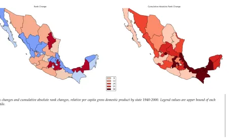
between the rank movements of the states. Figure 5 displays the spatial distribution of positional

change alongside the cumulative sum of absolute rank change over the entire 60 year period.

The latter measures the overall volatility in the rank movements of individual states. There is

no relationship between the volatility in a state’s position decade-to-decade and the magnitude

of the positional change in the income distribution over this period (ρ = 0.30, p = 0.10). The

two measures also display distinct spatial patterns, as the volatility of ranks is highly spatially

autocorrelated (I=0.33, p=0.01), while the end-point change is spatially random (I =0.03, p=

0.29).3 _{A more detailed spatiotemporal analysis of the rank dynamics necessitates the application}

of the LIMAs as shown in the following sections.

[Figure 3 about here.]

[Figure 4 about here.]

[Figure 5 about here.]

[Figure 6 about here.]

4.1. Global Autocorrelation and Global Mobility

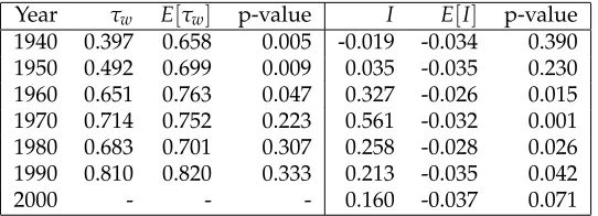
Table 1 summarizes the global measures of spatial autocorrelation and rank concordance over the

regions defined in Figure 6b. The complementary nature of the two statistics is reflected in the

significant spatial rank mobility found in the first three decades of the sample, as the degree of

rank concordance between neighboring pairs is significantly lower than what would be expected

under spatial randomness of rank changes. Coexisting with this rank mobility are spatially

random incomes in the first two decades with spatial autocorrelation becoming significant in 1960.

From 1970 forward the pattern switches to rank concordance that does not depart from spatial

randomness, in the sense that the concordance pattern for neighboring states is not distinguished

from that between states that are not neighbors, while the levels of income remains spatially

autocorrelated throughout 1970-2000.

[Table 1 about here.]

4.2. LIMAs

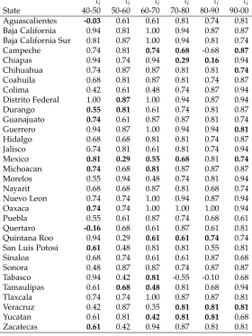
Local Concordanceτi:Table 2 reports the location specificτi values for each 10-year transitional

period, along with the results of a local indicator of spatial association for each value. Theτivalues

associated with a significant LISA are indicated in bold. Recall that theτireports the concordance

between a specific state’s income rank and the rest of the system, while the LISA asks if theseτi

values are locally clustered in space.

With regard to theτi values, concordance is the dominant pattern. This is seen, for example, in

Distro Federal for the 1940-50 period over which it does not swap ranks with any of the other states

(also see Figure 4). There are some exceptions, however, as both Aguacalientes and Queretaro have

negativeτi values in the first transitional period, indicating that they are sources of rank change

in the distribution. As was noted above, Campeche experienced the greatest upward movement

in the rank distribution over the entire period, yet examination of Table 2 reveals that much of

this movement was concentrated in the 1980-90 period as reflected in the strong negativeτi. The

localτi values can also vary in sign and magnitude for a given state over time. For example,

Campeche’s strong negative value in the 1980-90 period is bracketed by strong concordance values,

and a similar pattern can be seen for the state of Tabasco.

The local spatial association pattern of these state concordance values is also complex. The

bold values indicate significant LISA values for the specificτi but the nature of those spatial

values in 1940-50 for Aguacalientes and Queretaro, while the remaining significant LISAs are

all associated with positive τi values for the focal state. It is important to note; that, in the

former case the significant LISAs are pointing to spatial outliers - the strong negative concordance

values for Aguascalientes and Queretaro are significantly different from the concordance values in

their neighboring states. For other significant LISAs the pattern is of spatial value similarity for

the state-specific concordance values, whether those concordance values are strongly, or weakly,

positive. This indicates that, relative to the entire spatial distribution, these states generally hold

their rank positions. It does not necessarily imply that the concordance relationships between the

neighboring pairs are stable, however.

[Table 2 about here.]

Neighbor setτ˜i: Table 3 reports the values for the version of the LIMA based on the neighbor

set. Here the question is whether the concordance relationship between the focal state and its

neighbors is different from what could be expected from randomly distributed rank changes.

Inference is based on conditional randomization for each state under the null. That is, the sampling

distribution for the local ˜τiis obtained by randomly selectingnineighbors from the set ofnthat

excludesi and recalculating the statistic. This process is repeated 99 times for each state, and

pseudo p-values are obtained by comparing the observed statistic to this conditional distribution

under the null.

There are a number of interesting patterns that emerge from the table. The value for the LIMA

in Campeche is significant in four of the six transitional periods, three of which show concordance

while one displays discordance with its neighbors. In the discordant period Campeche has

swapped positions with all of its neighbors, again reflecting the period where it climbed up the

income distribution in rapid fashion. Thus, not only did it pass states that were not its geographical

neighbors (as was seen in the previous table), it also leapfrogged its geographical neighbors.

Another interesting case of local spatial dynamics is seen in Oaxaca situated in the poverty belt

of Mexico’s southern states. While the received wisdom is that southern states lag behind the rest

of the country, what has not been recognized is the complexity of the local spatial dynamics within

dominance. Distrito Federal maintains is position relative to its neighbors during each of the

transitional periods. However, its local value is significant in four, but not all, of the six transitions.

Even though the observed values are the same in all six years, the distribution of the local statistic

under the null is sensitive to the overall amount of concordance in the rank distribution over a

specific transition period.

[Table 3 about here.]

Neighborhood Set τ˜˜i: Table 4 reports the values for the version of the LIMA based on the

neighborhood set. Now the question is if the concordance relationships for a subset of states,

defined as the focal state and its neighbors, is different from what would be expected from

randomly distributed rank changes. In contrast to the previous LIMA where the concordance

relationship is viewed as a one-to-many (i.e., focal to each of its neighbors), here the local

concordance value is based on a many-to-many relationship. That is, the pairwise concordance

relations are measured for all pairs of states belonging to a focal state’s neighborhood set. Inference

is again based on conditional random permutations for each state.

A comparison of Tables 4 and 3 reveals a number of important differences in the local

concordance measures, as well as a few similarities. An important distinction is the non-negativity

of the local values for ˜˜τi in contrast to more instances of local discordance reported in Table 3.

One clear example of this is Campeche which goes from total local discordance in 1980-90

according to ˜τi, to a local concordance value of ˜˜τi = 0 during the same period when using

the neighborhood set basis. This implies that while Campeche leapfrogged all of its neighbors

during this transition period, the pattern of pairwise concordance between each of its neighbors

was a more mixed one with the number of concordant and discordant pairs counterbalancing

in Campeche’s neighborhood set. An explanation for the dominance of positive values for

neighborhood set LIMA in Table 4 is that the transitions are for a short 10-year period and the

number of concordance pairwise relations for members within a neighborhood set dominates the

fewer instances of pairwise discordance in the set.

In contrast to the case of Campeche, the values of the two types of LIMAs are identical for

Distrito Federal, pointing to absolute concordance between itself and its neighbors, but also

between all pairs of Distrito Federal’s neighbors. There is, however, a difference in the temporal

neighborhood set and the neighbor set constructs that define the two statistics.

It also important to note that the values for this second LIMA will be identical for all members

of a neighborhood set given that block weights are used. What may vary over the members of the

neighborhood set is the significance of the statistic because the permutations are conditional upon

the focal state under consideration. This is seen in the case of Mexico and Distrito Federal which

comprise the capital region.

The two sets of LIMAs thus provide complementary views on the local spatial dynamics, the

former yielding insights as to a focal state’s concordance relationships with its neighbors and the

latter describing the regional concordance dynamics surrounding the focal state.

[Table 4 about here.]

4.3. Interregional and Intraregional Mobility Decomposition

The results of applying the interregional concordance decomposition are reported in Table 5. The

diagonal elements report the amount of intraregional concordance in state incomes between 1940

and 2000, while the off-diagonal elements measure interregional concordance. Bold values indicate

statistical significance atp=0.05, where inference is based on random spatial permutations of the

state incomes. It is important to note that the global level of rank concordance remains constant

over the permutations. Thus, the null hypothesis here is whether the interregional or intraregional

concordance observed is significantly different from what would be expected if income mobility

were random in its spatial distribution.

The observed patterns of intraregional concordance do not depart from random values with

the exception of the Gulf region where the internal concordance value of 0.20 is significantly below

that observed under the null hypothesis of random spatial patterning of rank changes. Put another

way, the member states of the Gulf region exchange ranks more frequently with one another than

what would be expected by random chance.

In contrast to the intraregional concordance results, interregional rank mobility departs from

randomness more frequently. For example, states from the South and North regions never

experience pairwise exchange of ranks leading to significant concordance (lack of mobility) over

rank separation. Alongside these instances of rank concordance, there are two pairs of regions

that exhibit significant interregional exchange mobility, these are the Center and Gulf, and the

Center-N and North region. The case of the Center region thus illustrates that the decomposition

can illuminate meso-level pairwise interregional dynamics that may be masked by the global

mobility measure and not considered by the location specific indicators. Thus the interregional

and intraregional mobility decomposition provides a useful complement to the global and local

analytics.

[Table 5 about here.]

5. C

onclusion

This article has introduced a family of local indicators of mobility association that provide a number

of new perspectives on space-time dynamics. First, the LIMAs are directly linked to previously

developed global indicators of spatial concordance that identify hot-spots, and cold-spots, of

spatial change, together with locations that deviate from the overall general pattern of space-time

concordance. Second, the additive decomposition of the LIMAs permits the development of a

meso-level analytic to examine whether the overall space-time concordance is driven by interregional

or intraregional concordance. That is, are groups of observations (regions) displaying space-time

dynamics distinct from the global pattern? This adds an important dynamic complement to the

work on static decomposition of spatial inequality into its interregional and intraregional parts.

The initial application of these measures to the case study of Mexican state income dynamics

over the 1940-2000 period suggests that the LIMAs can provide new insights on regional income

distribution dynamics. At the same time, this is an initial foray into the LIMAs and much work

remains to be done. The LIMA statistics are designed to detect hot-spots of space-time concordance

and uncover interesting patterns in spatial pattern evolution. These are some of the goals of

exploratory space-time methods, which, in turn lead naturally to questions about the processes

may be responsible for the patterns uncovered. From a policy evaluation perspective there has

been a resurgence of interest in new methods to examine the impacts of “trickle-down” economic

policies on inequality and mobility (e.g. Bourguignon, 2011), and the LIMA’s offer a spatial lens

on these distributional questions. More broadly, the development of spatially explicit theories of

and Reed, 1990), the role of labor migration and changes in industrial composition (Crescenzi

et al., 2012), and to address the question of whether regional economic growth is competitive or

cooperative between neighboring regions (Chung and Hewings, 2015) are just a selection among

the numerous future avenues for confirmatory work that the new measures can afford.

From a more methodological perspective there are also several key areas for future research.

Thus far inference on the LIMAs has been based on conditional random spatial permutations which

provides one approach to assessing the statistical significance of the indicators. Computational

challenges associated with the global space-time concordance measure have been addressed (Rey,

2014) but need to be revisited in the local case since now conditional permutations are required.

The theoretical sampling distributions of the LIMA family also need to be examined. This is

particularly important as the LIMAs are a specific case of a local statistic, and thus face the same

challenges shared by all local statistics. These include the issues of multiple comparisons, the

lack of independence between the individual LIMAs, the distribution of the local statistics in the

presence of global space-time concordance, and the sensitivity of the statistic to the choice of

spatial weights matrix. Additionally, the developing composite measures of spatial dynamics that

combine changes in a global, and local, spatial autocorrelation statistics with the LIMAs presented

here is a promising direction for future research.

As the LIMAs are based on ranks the issues associated with the shift from an interval to

ordinal measurement scale raises the question of a trade-off between a potential loss of power and

a gain of generality. The generality arises from the relaxation of a number of potentially restrictive

assumptions underlying traditional correlation statistics. For example, in a space-time context the

analysis of change in absolute values of some series can be problematic, as in the case of remote

sensing data where direct comparison of illumination data from two different periods is difficult

without rank normalization of the data (Nelson et al., 2005). Similarly, rank distributions are

robust to extreme outliers that can have major impacts on interval correlation statistics. Moreover,

there is some evidence to suggest that the power of rank statistics can actually be quite high

(Kendall, 1962, p 166) so the trade-off between increased generalization and loss of power may not

be as great as first thought.

The avalanche of new types of spatio-temporal data associated with streaming sources (i.e., sensors,

geographical positioning systems, imagery, cell phones, etc.) appears to be an ideal domain for

the use of the LIMAs to identify space-time clustering, emergent properties, as well as rigidity

and inertia in space-time patterns. The LIMA’s have an interesting property that they can be

efficiently updated when new data become available unlike other space-time correlation measures

that would require complete recalculation.

Finally, while the current application relied on polygon data to illustrate the LIMAs and their

properties, the approach can easily be extended to any type of spatial support where neighbor

relationships between observational units can be defined. For example, LIMA’s could be applied

to the analysis of network constrained phenomena, such as traffic flows, or to marked point

patterns.4 Irrespective of the specific spatial support, the LIMAs could also be employed as part of

new data-driven approaches to delineate regions and/or to detect changes in region definitions

over time.

R

eferences

Anselin, L. (1995). Local indicators of spatial association-LISA.Geographical Analysis, 27(2):93–115.

Anselin, L. and Rey, S. J. (2014).Modern spatial econometrics in practice: A guide to GeoDa, GeoDaSpace

and PySAL. GeoDa Press.

Aroca, P., Bosch, M., and Maloney, W. F. (2005). Spatial dimensions of trade liberalization and

economic convergence: Mexico 1985–2002. The World Bank Economic Review, 19(3):345–378.

Beenstock, M. and Felsenstein, D. (2007). Mobility and mean reversion in the dynamics of regional

inequality. International Regional Science Review, 30(4):335–361.

Bigman, D. and Srinivasan, P. (2002). Geographical targeting of poverty alleviation programs:

methodology and applications in rural India. Journal of Policy Modeling, 24(3):237–255.

Bourguignon, F. (2011). Non-anonymous growth incidence curves, income mobility and social

welfare dominance. The Journal of Economic Inequality, 9(4):605–627.

Chetty, R., Hendren, N., Kline, P., and Saez, E. (2014). Where is the land of opportunity? The

geography of intergenerational mobility in the United States. Technical report, National Bureau

of Economic Research.

Chung, S. and Hewings, G. J. (2015). Competitive and complementary relationship between

regional economies: a study of the Great Lake States.Spatial Economic Analysis, 10(2):205–229.

Cramer, C. (2003). Does inequality cause conflict? Journal of International Development, 15(4):397–412.

Crescenzi, R., Rodríguez-Pose, A., and Storper, M. (2012). The territorial dynamics of innovation

in China and India.Journal of Economic Geography, 12(5):1055–1085.

Cuadrado-Roura, J. R. (2009). Regional policy, economic growth and convergence: lessons from the

Spanish case. Springer Verlag.

Esquivel, G. (1999). Convergencia regional en México, 1940-1995. El trimestre económico, (264):725.

Fields, G. (2010). Does income mobility equalize longer-term incomes? New measures of an old

concept. Journal of Economic Inequality, 8(4):409–427.

Formby, J., Smith, W., and Zheng, B. (2004). Mobility measurement, transition matrices and

statistical inference.Journal of Econometrics, 120(1):181–205.

Hammond, G. W. and Thompson, E. (2006). Convergence and mobility: Personal income trends in

US metropolitan and nonmetropolitan regions.International Regional Science Review, 29(1):35–63.

Jalan, J. and Ravallion, M. (1998). Are there dynamic gains from a poor-area development program?

Journal of Public Economics, 67(1):65–85.

Kanbur, S. and Venables, A. (2005). Spatial inequality and development. Oxford University Press,

USA.

Kendall, M. G. (1962). Rank correlation methods. Griffin, London, 3rd edition.

Le Gallo, J. (2004). Space-time analysis of GDP disparities across European regions: a Markov

criteria for determining leading regions in wage transmission models. Journal of Regional Science,

30(1):37–50.

Maasoumi, E. (1998). On mobility.Handbook of applied economic statistics, pages 119–175.

Maasoumi, E., Racine, J., and Stengos, T. (2007). Growth and convergence: A profile of distribution

dynamics and mobility. Journal of Econometrics, 136(2):483–508.

Magrini, S. (1999). The evolution of income disparities among the regions of the European Union.

Regional Science and Urban Economics, 29(2):257–281.

Nelson, T., Wilson, H., Boots, B., and Wulder, M. (2005). Use of ordinal conversion for radiometric

normalization and change detection. International Journal of Remote Sensing, 26(3):535–541.

Partridge, M. D. (1997). Is inequality harmful for growth? Comment. The American Economic

Review, pages 1019–1032.

Piketty, T. (2014). Capital in the Twenty-first Century. Harvard University Press.

Quah, D. T. (1996a). Empirics for economic growth and convergence. European Economic Review,

40(6):1353–1375.

Quah, D. T. (1996b). Twin peaks: Growth and convergence in models of distribution dynamics.

The Economic Journal, 106:1045–1055.

Rey, S. J. (2001). Spatial empirics for economic growth and convergence. Geographical Analysis,

33(3):195–214.

Rey, S. J. (2004). Spatial analysis of regional income inequality. In Goodchild, M. and Janelle,

D., editors,Spatially Integrated Social Science: Examples in Best Practice, pages 280–299. Oxford

University Press, Oxford.

Rey, S. J. (2014). Fast algorithms for a space-time concordance measure. Computational Statistics,

29(3-4):799–811.

Rey, S. J. (2016). Bells in space: The spatial dynamics of US interpersonal and interregional income

Rey, S. J. and Anselin, L. (2007). PySAL: A Python library of spatial analytical methods.The Review

of Regional Studies, 37(1):5–27.

Rey, S. J. and Montouri, B. D. (1999). U.S. regional income convergence: A spatial econometric

perspective. Regional Studies, 33(2):145–156.

Rey, S. J. and Sastré-Gutiérrez, M. L. (2010). Interregional inequality dynamics in Mexico. Spatial

Economic Analysis, 5(3):277–298.

Schluter, C. (1998). Statistical inference with mobility indices. Economics letters, 59(2):157–162.

Schorrocks, A. (1978). Income inequality and income mobility.Journal of Economic Theory, 19:376–

393.

Shorrocks, A. and Wan, G. (2005). Spatial decomposition of inequality. Journal of Economic

Geography, 5(1):59–81.

Stiglitz, J. (2012). The price of inequality. Penguin UK.

The Economist (2011). Regional inequlity: The gap between many rich and poor regions widened

because of the recession. http://www.economist.com/node/18332880?story_id=18332880.

Webber, D., White, P., and Allen, D. (2005). Income convergence across US States: An analysis

using measures of concordance and discordance.Journal of Regional Science, 45(3):565–589.

SERGIO REY is a Professor in the School of Geographical Sciences and Urban Planning at Arizona

State University, Tempe, AZ 85287. E-mail: [email protected]. His research interests include

spatio-temporal data analysis, geocomputation, geovisualization, regional inequality dynamics, open

L

ist of

F

igures

1 Global Indicator of Rank Mobility: Case I . . . 26 2 Global Indicator of Rank Mobility: Case II . . . 27 3 Relative per capita gross domestic product by state 1940-2000. Legend values are

upper bound of each quintile. . . 28 4 Spaghetti Plot, relative incomes Mexican States 1940-2000 . . . 29 5 Rank changes and cumulative absolute rank changes, relative per capita gross

1 2 5 6

3 4 7 8

9 10 13 14 11 12 15 16

(a)Ranks period t0

1 2 5 6

3 4 7 8

9 10 16 15 11 12 14 13

(b)Ranks period t1

0 0 1 1 0 0 1 1 2 2 3 3 2 2 3 3

(c)Regimes

1 2 5 6

3 4 7 8

9 10 13 14 11 12 15 16

(a)Ranks period t0

5 6 1 2

7 8 3 4

13 14 9 10 15 16 11 12

(b)Ranks period t1

0 0 1 1 0 0 1 1 2 2 3 3 2 2 3 3

(c)Regimes

(a)Mexican States

(b)Mexican regions after Esquivel (1999)

L

ist of

T

ables

1 Global Concordance and Spatial Autocorrelation . . . 33 2 Location specificτi. Bold values indicate significant LISA statistics for the associated

τi. . . 34

3 Neighbor set Local Indicators of Mobility Association: ˜τi. Bold values are statistically

significant at p=0.05. . . 35 4 Neighborhood set Local Indicators of Mobility Association: ˜˜τi. Bold values are

statistically significant at p=0.05. . . 36 5 Inter and Intraregional Concordance Decomposition 1940-2000. Values on the

Year τw E[τw] p-value I E[I] p-value

1940 0.397 0.658 0.005 -0.019 -0.034 0.390 1950 0.492 0.699 0.009 0.035 -0.035 0.230 1960 0.651 0.763 0.047 0.327 -0.026 0.015 1970 0.714 0.752 0.223 0.561 -0.032 0.001 1980 0.683 0.701 0.307 0.258 -0.028 0.026 1990 0.810 0.820 0.333 0.213 -0.035 0.042 2000 - - - 0.160 -0.037 0.071

τi τi τi τi τi τi

State 40-50 50-60 60-70 70-80 80-90 90-00 Aguascalientes -0.03 0.61 0.61 0.81 0.74 0.81 Baja California 0.94 0.81 1.00 0.94 0.87 0.87 Baja California Sur 0.81 0.87 1.00 0.94 0.81 0.74 Campeche 0.74 0.81 0.74 0.68 -0.68 0.87

Chiapas 0.94 0.74 0.94 0.29 0.16 0.94 Chihuahua 0.74 0.87 0.87 0.81 0.81 0.74

Coahuila 0.68 0.81 0.87 0.81 0.74 0.87 Colima 0.42 0.61 0.48 0.74 0.87 0.94 Distrito Federal 1.00 0.87 1.00 0.94 0.87 0.94 Durango 0.55 0.81 0.61 0.74 0.81 0.87 Guanajuato 0.74 0.61 0.87 0.87 0.81 0.74 Guerrero 0.94 0.87 1.00 0.94 0.94 0.81

Hidalgo 0.68 0.68 0.81 0.81 0.74 0.87 Jalisco 0.74 0.81 0.61 0.81 0.74 0.94 Mexico 0.81 0.29 0.55 0.68 0.81 0.74

Michoacan 0.74 0.68 0.81 0.87 0.87 0.87 Morelos 0.55 0.94 0.48 0.74 0.81 0.94 Nayarit 0.68 0.68 0.87 0.81 0.68 0.74 Nuevo Leon 0.74 0.74 1.00 0.94 0.87 0.94 Oaxaca 0.74 0.74 1.00 1.00 1.00 0.94 Puebla 0.55 0.61 0.87 0.74 0.68 0.61 Quertaro -0.16 0.68 0.61 0.87 0.61 0.81 Quintana Roo 0.94 0.29 0.61 0.61 0.74 0.74 San Luis Potosi 0.61 0.48 0.81 0.81 0.55 0.81 Sinaloa 0.68 0.74 0.61 0.61 0.87 0.68 Sonora 0.48 0.87 0.87 0.74 0.87 0.87 Tabasco 0.94 0.42 0.81 -0.55 -0.10 0.68 Tamaulipas 0.61 0.68 0.48 0.81 0.68 0.94 Tlaxcala 0.74 0.74 1.00 0.87 0.87 0.81 Veracruz 0.42 0.87 0.35 0.81 0.81 0.81

Yucatan 0.61 0.81 0.42 0.81 0.81 0.68 Zacatecas 0.61 0.42 0.94 0.87 0.81 0.81

˜

τr τ˜r τ˜r τ˜r τ˜r τ˜r

State 40-50 50-60 60-70 70-80 80-90 90-00 Aguascalientes -0.20 0.20 0.60 1.00 0.60 0.60 Baja California 1.00 0.60 1.00 1.00 1.00 0.60 Baja California Sur 1.00 1.00 1.00 1.00 1.00 1.00 Campeche 1.00 0.50 0.50 0.50 -1.00 1.00 Chiapas 0.33 -0.33 0.33 0.33 -0.33 0.33

Chihuahua 0.60 0.60 0.20 0.60 1.00 0.20

Coahuila 0.60 0.60 0.20 0.60 1.00 0.60 Colima -0.50 1.00 0.50 0.50 1.00 1.00 Distrito Federal 1.00 1.00 1.00 1.00 1.00 1.00

Durango 1.00 1.00 0.20 1.00 1.00 1.00 Guanajuato 0.20 0.20 0.60 1.00 0.60 1.00

Guerrero 0.33 0.33 1.00 1.00 0.33 1.00

Hidalgo 0.33 1.00 1.00 1.00 0.33 0.33 Jalisco 0.50 1.00 1.00 1.00 1.00 1.00 Mexico 1.00 1.00 1.00 1.00 1.00 1.00 Michoacan 1.00 0.33 0.33 0.33 0.33 1.00

Morelos 1.00 1.00 1.00 1.00 1.00 1.00 Nayarit 0.00 0.50 0.50 1.00 1.00 1.00

Nuevo Leon 0.60 0.20 1.00 1.00 1.00 1.00 Oaxaca -0.33 -0.33 1.00 1.00 1.00 0.33

Puebla -0.33 1.00 1.00 1.00 0.33 0.33 Quertaro -0.60 0.20 0.20 1.00 0.60 0.60 Quintana Roo 1.00 0.00 0.00 0.50 0.00 1.00 San Luis Potosi 0.20 -0.20 1.00 1.00 0.60 1.00

Sinaloa 0.00 0.50 1.00 0.50 1.00 1.00

Sonora 0.20 0.60 0.20 0.20 1.00 1.00 Tabasco 1.00 0.50 0.50 -1.00 0.00 0.50 Tamaulipas 0.60 1.00 1.00 1.00 1.00 1.00 Tlaxcala 0.33 1.00 1.00 1.00 1.00 1.00

Veracruz 0.50 0.50 0.50 0.00 0.50 1.00

Yucatan 0.50 0.50 0.50 0.00 0.50 0.50 Zacatecas -0.20 -0.20 1.00 1.00 1.00 1.00

˜˜

τr τ˜˜r τ˜˜r τ˜˜r τ˜˜r τ˜˜r

State 40-50 50-60 60-70 70-80 80-90 90-00 Aguascalientes 0.07 0.20 0.60 1.00 0.73 0.87 Baja California 0.60 0.60 0.60 0.73 1.00 0.73 Baja California Sur 0.20 0.80 0.80 0.80 1.00 1.00 Campeche 0.80 0.40 0.40 0.00 0.00 0.80 Chiapas 0.33 0.00 0.67 0.67 0.33 0.67

Chihuahua 0.60 0.60 0.60 0.73 1.00 0.73 Coahuila 0.60 0.60 0.60 0.73 1.00 0.73 Colima 0.20 0.80 0.80 0.80 1.00 1.00 Distrito Federal 1.00 1.00 1.00 1.00 1.00 1.00

Durango 0.07 0.20 0.60 1.00 0.73 0.87 Guanajuato 0.07 0.20 0.60 1.00 0.73 0.87 Guerrero 0.33 0.00 0.67 0.67 0.33 0.67 Hidalgo 0.33 1.00 1.00 1.00 0.67 0.67 Jalisco 0.20 0.80 0.80 0.80 1.00 1.00 Mexico 1.00 1.00 1.00 1.00 1.00 1.00 Michoacan 0.33 0.00 0.67 0.67 0.33 0.67 Morelos 0.33 1.00 1.00 1.00 0.67 0.67 Nayarit 0.20 0.80 0.80 0.80 1.00 1.00 Nuevo Leon 0.60 0.60 0.60 0.73 1.00 0.73 Oaxaca 0.33 0.00 0.67 0.67 0.33 0.67 Puebla 0.33 1.00 1.00 1.00 0.67 0.67 Quertaro 0.07 0.20 0.60 1.00 0.73 0.87 Quintana Roo 0.80 0.40 0.40 0.00 0.00 0.80 San Luis Potosi 0.07 0.20 0.60 1.00 0.73 0.87 Sinaloa 0.20 0.80 0.80 0.80 1.00 1.00 Sonora 0.60 0.60 0.60 0.73 1.00 0.73 Tabasco 0.80 0.40 0.40 0.00 0.00 0.80 Tamaulipas 0.60 0.60 0.60 0.73 1.00 0.73 Tlaxcala 0.33 1.00 1.00 1.00 0.67 0.67 Veracruz 0.80 0.40 0.40 0.00 0.00 0.80 Yucatan 0.80 0.40 0.40 0.00 0.00 0.80 Zacatecas 0.07 0.20 0.60 1.00 0.73 0.87

Table 4:Neighborhood set Local Indicators of Mobility Association: τ˜˜_i. Bold values are statistically significant at

Capital Center Center-N Gulf North Pacific South Capital 1.00 0.25 0.50 0.60 0.83 0.60 1.00 Center 0.25 0.33 0.50 0.30 0.92 0.40 0.75 Center-N 0.50 0.50 0.60 0.40 0.39 0.53 0.83 Gulf 0.60 0.30 0.40 0.20 0.40 0.28 0.80 North 0.83 0.92 0.39 0.40 0.60 0.73 1.00

Pacific 0.60 0.40 0.53 0.28 0.73 0.80 0.80 South 1.00 0.75 0.83 0.80 1.00 0.80 0.33

Table 5:Inter and Intraregional Concordance Decomposition 1940-2000. Values on the diagonal are the intraregional