Automatic Inference of Sound Correspondence Patterns across Multiple Languages

Correspondence Patterns across

Multiple Languages

Johann-Mattis List

Department of Linguistic and Cultural Evolution, Max Planck Institute for the Science of Human History, Jena

Sound correspondence patterns play a crucial role for linguistic reconstruction. Linguists use them to prove language relationship, to reconstruct proto-forms, and for classical phylogenetic reconstruction based on shared innovations. Cognate words that fail to conform with expected patterns can further point to various kinds of exceptions in sound change, such as analogy or assimilation of frequent words. Here I present an automatic method for the inference of sound correspondence patterns across multiple languages based on a network approach. The core idea is to represent all columns in aligned cognate sets as nodes in a network with edges representing the degree of compatibility between the nodes. The task of inferring all compatible correspondence sets can then be handled as the well-known minimum clique cover problem in graph theory, which essentially seeks to split the graph into the smallest number of cliques in which each node is represented by exactly one clique. The resulting partitions represent all correspondence patterns that can be inferred for a given data set. By excluding those patterns that occur in only a few cognate sets, the core of regularly recurring sound correspondences can be inferred. Based on this idea, the article presents a method for automatic correspondence pattern recognition, which is implemented as part of a Python library which supplements the article. To illustrate the usefulness of the method, I present how the inferred patterns can be used to predict words that have not been observed before.

1. Introduction

By comparing the languages of the world, we gain invaluable insights into human prehistory, predating the appearance of written records by thousands of years. The clas-sical methods for historical language comparison, a collection of different techniques summarized under the termcomparative method(Meillet 1954; Weiss 2015), date back to the early 19th century and have since then been constantly refined and improved (see Ross and Durie 1996 for details on the practical workflow). Thanks to the comparative method, linguists have made groundbreaking insights into language change in general and into the history of many specific language families (Campbell and Poser 2008) and external evidence has often confirmed the validity of the findings (McMahon and

Submission received: 4 April 2018; revised version received: 3 October 2018; accepted for publication: 21 November 2018.

McMahon 2005, pages 10–14). With increasing amounts of data, however, the methods, which are largely manually applied, reach their practical limits. As a result, scholars are now increasingly trying to automate different aspects of the classical comparative methods (Kondrak 2000; Proki´c, Wieling, and Nerbonne 2009; List 2014).

One of the fundamental insights of early historical linguistic research was that— as a result of systemic changes in the sound system of languages—genetically related languages exhibit structural similarities in those parts of their lexicon that were com-monly inherited from their ancestral languages. These similarities surface in the form of

correspondence relationsbetween sounds from different languages in cognate words. English th [θ], for example, is usually reflected as d in German, as we can see from cognate pairs like English thinkversus German denken, or English thorn and German Dorn. Englisht, on the other hand, is usually reflected asz[ts]in German, as we can see from pairs like Englishtoeversus GermanZeh, or Englishtenversus Germanzehn. The identification of theseregular sound correspondencesplays a crucial role in historical language comparison, serving not only as the basis for the proof of genetic relationship (Dybo and Starostin 2008; Campbell and Poser 2008) or the reconstruction of proto-forms(Hoenigswald 1960, pages 72–85; Anttila 1972, pages 229–263), but (indirectly) also for classical subgrouping based on shared innovations (which would not be possi-ble without identified correspondence patterns).

With the beginning of this millennium, historical linguistics has witnessed an increased number of attempts to quantify specific tasks of the traditional compar-ative method. Since then, scholars have repeatedly attempted to either directly in-fer regular sound correspondences across genetically related languages (Kay 1964; Brown, Holman, and Wichmann 2013; Kondrak 2003, 2009) or integrated the infer-ence into workflows for automatic cognate detection (Guy 1994; List 2012, 2014; List, Greenhill, and Gray 2017). What is interesting in this context, however, is that almost all approaches dealing with regular sound correspondences, be it early formal—but clas-sically grounded—accounts (Grimes and Agard 1959; Hoenigswald 1960) or computer-based methods (Kondrak 2002, 2003; List 2014) only consider sound correspondences betweenpairsof languages.

A rare exception can be found in the work of Antilla (1972, pages 229–263) who presents the search for regular sound correspondences across multiple languages as the basic technique underlying the comparative method for historical language com-parison. Anttila’s description starts from a set of cognate word forms (or morphemes) across the languages under investigation. These words are then arranged in such a way that corresponding sounds in all words are placed into the same column of a matrix. The extraction of regularly recurring sound correspondences in the languages under investigation is then based on the identification of similar patterns recurring across different columns within the cognate sets. The procedure is illustrated in Figure 1, where four cognate sets in Sanskrit, Ancient Greek, Latin, and Gothic are shown, two taken from Anttila (1972, page 246) and two added by me.

Two points are remarkable about Anttila’s approach. First, it builds heavily on the

phonetic alignmentof sound sequences,1_{by which the sound sequences of words are} arranged in a matrix in such a way that all corresponding sounds are placed in the same cell (List 2014). Second, it reflects a concrete technique by which regular sound

A B C D E F

Sanskrit y u g a m dh u h i (tar) s n u ṣ (ā) - r u dh (iras) Greek z u g o n th u g a (ter-) - n u - (os) e r u th (rós) Latin i u g u m Ø Ø Ø Ø (Ø) - n u r (us) - r u b (er) Gothic j u k - - d au h - (tar) Ø Ø Ø Ø (Ø) Ø Ø Ø Ø (Ø)

Gloss 'yoke' 'daughter' 'daughter-in-law' 'red'

Figure 1

Regular sound correspondences across four Indo-European languages, illustrated with help of alignments along the lines of Anttila (1972, page 246). In contrast to the original illustration, lost sounds are displayed with help of the dash “-” as a gap symbol, while missing words (where no reflex in Gothic or Latin could be found) are represented by the “∅” symbol.

correspondences for multiple languages can be detected and employed as a starting point for linguistic reconstruction. If we look at the framed columns in the four exam-ples in Figure 1, which are further labeled alphabetically, we can easily see that the patterns A, E, and F are remarkably similar. The only difference is that we miss data for Gothic in the patterns E and F, and, as a result, we don’t havereflex sounds(sounds in a given alignment column as reflected in a cognate word) for the full sound correspon-dence patterns in the respective columns. The same holds, however, for columns C, E, and F. Since A and C differ regarding the reflex sound of Gothic (uvs.au), they cannot be assigned to the same correspondence set at this stage, and if we want to solve the problem of finding the regular sound correspondences for the words in the figure, we need to decide which columns in the alignments we assign to the same correspondence set, thereby “imputing” missing sounds where we miss a reflex. Assuming that the “regular” pattern in our case is reflected by the group of C, E, and F, we can make predictionsabout the sounds missing in Gothic in E and F, concluding that, if ever we find the missing reflex in so far unrecognized sources of Gothic in the future, we would expect a-au-in the words for “daughter-in-law” and “red”.2

We can easily see how patterns of sound correspondences across multiple languages can serve as the basis for multiple tasks in historical linguistics. First, we could use them to guess how a word that is missing in a given alignment would sound in that language, if it could be found. Since the task of identifying cognate words across multi-ple languages is very commulti-plex, and words may have drastically shifted their meanings, we could use the predictions to search for missing cognate forms in those areas of the lexicon that we have not considered before.3 _{Second, if two alignment columns are} identical, they must reflect the same proto-sound, if alternative processes like borrowing can be excluded. Thus, similarly to the prediction of missing words in our cognate sets, we could use correspondence patterns to infer proto-forms, provided that parts of the data are already annotated.4_{Third, we could use them to check linguistic claims}

2 As pointed out by the anonymous reviewer, Gothicráupsis a reflex of ‘red’ (Wright 1910, page 340), but as mentioned by Eugen Hill (personal communication), the Gothic form reflects a derivationally different formation and was therefore correctly not listed in Anttila’s examples.

3 Consider cases of shifted meanings like Englishhoundvs. GermanHund‘dog,’ or English-thorpas a prefix in place names compared to GermanDorf‘village.’

about cognate words themselves: If it turns out that the aligned cognate sets proposed by linguists do not pattern into recurring correspondences across the languages under consideration, we can directly criticize both individual claims regarding word relations and general claims about the genetic relation of languages.

While it seems trivial to identify sound correspondences across multiple languages from the few examples provided in Figure 1, the problem can become quite complicated if we add more cognate sets and languages to the comparative sample. Especially the handling ofmissing reflexesfor a given cognate set becomes a problem here, as missing data makes it difficult for linguists to decide which alignment columns to group with each other. This can already be seen from the examples given in Figure 1, where we have two possibilities to group the patterns A, C, E, and F, if we base our judgments only on these four patterns: E and F could be grouped with either A or C, and it may even be possible that one should be grouped with A and one with C. The “true” solution here depends on the history of the languages, but if the data that would allow us to reconstruct this history is lost, we can never infer the historically correct grouping with full confidence.

The goal of this article is to illustrate how a manual analysis in the spirit of Anttila can be automated and fruitfully applied—not only in purely computational approaches to historical linguistics, but also in computer-assisted frameworks that help linguists to explore their data before they start carrying out painstaking qualitative comparisons (List 2016). In order to illustrate how this problem can be solved computationally, the article will first discuss some important general aspects of sound correspondences and sound correspondence patterns in Section 2, introducing specific terminology that will be needed in the remainder. In Section 3, we will see that the problem of finding sound correspondences across multiple languages can be modeled as the well-known clique-cover problemin an undirected network (Bhasker and Samad 1991). While this problem is hard to solve in an exact way computationally,5 _{fast approximate solutions exist} (Welsh and Powell 1967) and can be easily applied. Based on these findings, the article will introduce a fully automated method for the recognition of sound correspondence patterns across multiple languages (Section 4). This method is implemented in the form of a Python library and can be readily applied to multilingual wordlist data as it is also required by software packages such as LingPy (List, Greenhill, and Forkel 2017) or software tools such as EDICTOR (List 2017). Section 5 will then illustrate how the method can be applied by testing how it performs in the task of predicting missing cognate words and missing proto-forms.

2. Preliminaries on Sound Correspondence Patterns

In the introduction, it was emphasized that the traditional comparative method is itself less concerned with regular sound correspondences attested for language pairs, but for all languages under consideration. In the following, this claim will be further substantiated, while at the same time introducing some major methodological consid-erations and ideas that are important for the development of the new method for sound correspondence pattern recognition.

Table 1

Comparing correspondence patterns for Proto-Germanic reflexes of*d-,*þ-, and*t-in German, English, and Dutch (Germanic proto-forms follow Kroonen [2013]).

2.1 From Sound Correspondences to Sound Correspondence Patterns

Sound correspondences are most easily defined for pairs of languages. Thus, it is straightforward to state that German[d]regularly corresponds to English[θ](or[ð]),

that German[ts]regularly corresponds to English[t], and that German[t]corresponds to English [d]. We can likewise expand this view to multiple languages by adding another Germanic language, such as, for example, Dutch to our comparison, which has

[d]in the case of German[d]and English [θ],[t]in the case of German[ts]and English

[t], and[d]in the case of German[t]and English[d].

The more languages and examples we add to the sample, however, the more com-plex the picture becomes, and while we can state three (basic) patterns for the case of English, German, and Dutch, given in our example, we may get easily more patterns, due to secondary sound changes in the different languages, although we would still reconstruct only three sounds in the proto-language ([θ, t, d]). This is illustrated in Table 1, where Proto-Germanic forms containing *p[þθ], *t, and *d in different pho-netic environments are contrasted with their descendant forms in German, English, and Dutch. The example shows that there is a one-to-n relationship between what we interpret as a proto-sound of the proto-language, and the regular correspondence patterns that we may find in our data. While we will reserve the termsound correspon-dencefor pairwise language comparison, we will use the termsound correspondence pattern(or simply correspondence pattern) for the abstract notion of regular sound correspondences across a set of languages that we can find in the data.

2.2 Correspondence Patterns in the Classical Literature

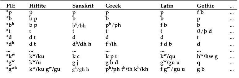
Table 2

Sound correspondence patterns for Indo-European stops, following Clackson (2007, page 37) .

PIE Hittite Sanskrit Greek Latin Gothic ...

*p p p p p f b ...

*b b p b b b p ...

*bh _{b p p}h_{/ph f b b ...}

*t t t t t θ/þ d ...

*d d t d d d t ...

*dh _{d t d}h_{/dh h t}h_{/th f d b d ...}

... ... ... ... ... ... ...

*kw _kw_{/ku k c k p t k}w_{/qu h}w_{/hw g ...}

*gw _kw_{/u g j g b d g}w_{/gu u q ...}

*gwh _kw_{/ku g}w_{/gu p}h_{/ph t}h_{/th k}h_{/kh f g}w_{/gu u g b ...}

correspondences in short form”.6_{However, given the one-to-nrelation between} proto-sounds and correspondence patterns, it is clear that this is not quite correct. Having inferred regular correspondence patterns in our data, our reconstructions will add a different level of analysis by furtherclusteringthese patterns into groups that we believe to reflect one single sound in the ancestral language.

That there are usually more than just one correspondence pattern for a recon-structed proto-sound is nothing new to most practitioners of linguistic reconstruction. Unfortunately, however, linguists rarely list all possible correspondence patterns ex-haustively when presenting their reconstructions, but instead select the most frequent ones, leaving the explanation of weird or unexpected patterns to comments written in prose. A first and important step of making a linguistic reconstruction system trans-parent, however, should start from an exhaustive listing of all correspondence patterns, including irregular patterns that occur very infrequently but would still be accepted by the scholars as reflecting true cognate words.

What scholars do instead is provide tables that summarize the correspondence patterns in a rough form, for example, by showing the reflexes of a given proto-sound in the descendant languages in a table, where multiple reflexes for one and the same language are put in the same cell. An example, taken with modifications7 _from Clackson (2007, page 37), is given in Table 2. In this table, the major reflexes of Proto-Indo-European stops in 11 languages representing the oldest attestations and major branches of Indo-European are listed. This table is a very typical example for the way in which scholars discuss, propose, and present correspondence patterns in linguistic reconstruction (Beekes 1995; Brown et al. 2011; Holton et al. 2012; Jacques 2017). The shortcomings of this representation become immediately transparent. Neither are we told about the frequency by which a given reflex is attested to occur in the descendant languages, nor are we told about the specific phonetic conditions that have been proposed to trigger the change where we have two reflexes for the same proto-sound.

6 My translation, original text: ‘Les «restitutions» ne sont rien autre chose que les signes par lesquels on exprime en abrégé les correspondances.’

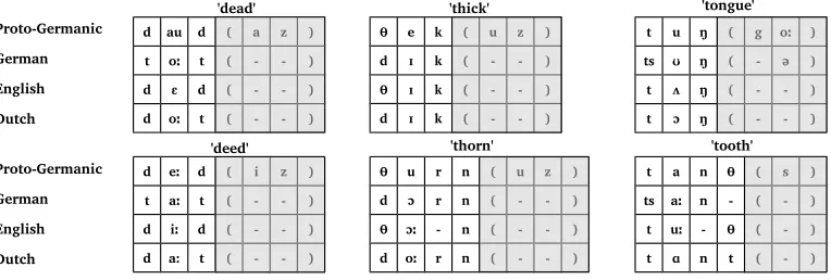
Proto-Germanic German English Dutch

Proto-Germanic German English Dutch

'dead' 'thick' 'tongue'

'deed' 'thorn' 'tooth'

d au d ( a z )

t oː t ( - - )

d ɛ d ( - - )

d oː t ( - - )

θ e k ( u z )

d ɪ k ( - - )

θ ɪ k ( - - )

d ɪ k ( - - )

t u ŋ ( g oː )

ts ʊ ŋ ( - ə )

t ʌ ŋ ( - - )

t ɔ ŋ ( - - )

d eː d ( i z ) t aː t ( - - ) d iː d ( - - )

d a: t ( - - )

θ u r n ( u z )

d ɔ r n ( - - )

θ ɔː - n ( - - )

d oː r n ( - - )

t a n θ ( s )

ts aː n - ( - ) t uː - θ ( - )

t ɑ n t ( - )

Figure 2

Alignment analyses of the six cognate sets from Table 1. Brackets around subsequences indicate that the alignments cannot be fully resolved due to secondary morphological changes.

While scholars of Indo-European tend to know these conditions by heart, it is perfectly understandable why they would not list them. However, when presenting the results to outsiders to their field in this form, it makes it quite difficult for them to correctly evaluate the findings. A sound correspondence table may look impressive, but it is of no use to people who have not studied the data themselves.

A further problem in the field of linguistic reconstruction is that scholars barely discuss workflows or procedures by which sound correspondence patterns can be inferred. For well-investigated language families like Indo-European or Austronesian, which have been thoroughly studied for more than one hundred years (Blust 1990), it is clear that there is no direct need to propose a heuristic procedure, given that the major patterns have been identified long ago and the research has reached a stage where scholarly discussions circle around individual etymologies or higher levels of linguistic reconstruction, like semantics, morphology, and syntax.8 _{For languages whose history} is less well known and where historical language reconstruction has not even reached a stage of reconstruction where a majority of scholars agree, however, a procedure that helps to identify the major correspondence patterns underlying a given data set would surely be incredibly valuable.

2.3 Correspondence Patterns and Alignments

In order to infer correspondence patterns, the data must be available inaligned form

(see Section 1), that is, we must know which of the sound segments that we compare across cognate sets are assumed to go back to the same ancestral segment. This is illustrated in Figure 2 where the cognate sets from Table 1 are presented inaligned form, with zero-matches (gaps) being represented as a dash ("-"), and with brackets indicating unalignable parts in the sequences, that is, parts that cannot be aligned, since the differences are not due to regular sound change.9 Although alignments are never explicitly mentioned in Clackson (2007), they are implied by the provided

8 For examples, compare the very detailed etymological discussions by Meier-Brügger (2002, pages 173–187).

θ u r n ( u z )

d ɔ r n ( - - )

θ ɔː - n ( - - )

d oː r n ( - - )

'thorn'

alignment site sound

correspondence pattern

θ e k ( u z )

d ɪ k ( - - )

θ ɪ k ( - - )

d ɪ k ( - - )

'thick'

Proto-Germanic German

English Dutch

θ d θ d

θ u r p ( a )

Ø Ø Ø Ø Ø Ø Ø

d ɔ r f ( - )

d ɔ r p ( - )

'thorp'

Figure 3

Alignment sites and correspondence patterns: While alignment sites are concrete representations of the presumed relations among cognate words, correspondence patterns are a further stage of abstraction.

correspondence patterns, which are presumably derived from the alignment of reflexes in each of the daughter languages. These assumed alignments are given in Table 2.

Following evolutionary biology, a given column of an alignment is called an align-ment site (or simply a site). An alignment site may reflect the same values as we find in a correspondence pattern, and correspondence patterns are usually derived from alignment sites, but in contrast to a correspondence pattern, an alignment site may reflect a correspondence pattern only incompletely, due to missing data in one or more of the languages under investigation. For example, when comparing German Dorf “village” with Dutch dorp , it is immediately clear that the initial sounds of both words represent the same correspondence pattern as we find for the cognate sets for “thick” and “thorn” given in Figure 2, although no reflex of their Proto-Germanic ancestor formþurpa-(originally meaning “crowd,” see Kroonen [2013, 553]) has survived in Modern English.10 Thanks to the correspondence patterns in Table 1, however, we know that—if we project the word back to Proto-Germanic—we must reconstruct the initial with *þ- ‘[θ], since the match of Germand-and Dutchd-occurs—if we ignore recent borrowings—only in correspondence patterns in which English hasth-.

These “gaps” due to missing reflexes of a given cognate set are not the same as the gaps inside an alignment, since the latter are due to the (regular) loss or gain of a sound segment in a given alignment site, while gaps due to missing reflexes may either reflect processes oflexical replacement(List 2014, page 37f), or a preliminary stage of research resulting from insufficient data collections or insufficient search for potential reflexes. While we use the dash as a symbol for gaps in alignment sites, we will use the character Ø(denoting the empty set) to represent missing data in correspondence patterns and alignment sites. The relation between correspondence patterns in the sense developed here and alignment sites is illustrated in Figure 3, where the initial alignment sites of three alignments corresponding to Proto-Germanic *þ [θ] are assembled to form one correspondence pattern.

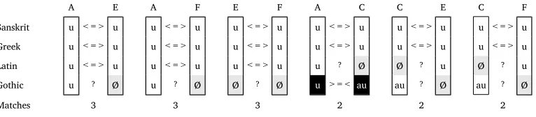
A E A F E F A C C E C F Sanskrit u <=> u --- u <=> u --- u <=> u --- u <=> u --- u <=> u --- u <=> u Greek u <=> _{u u} <=> _{u u} <=> _{u u} <=> _{u u} <=> _{u u} <=> _u

Latin u <=> u u <=> u u <=> u u ? Ø Ø ? u Ø ? u

Gothic u ? Ø u ? Ø Ø ? Ø u >=<au au ? Ø au ? Ø

Matches 3 3 3 2 2 2

Figure 4

Assessing the compatibility of the four alignment sites from Figure 1.

3. Preliminary Thoughts on Correspondence Pattern Recognition

If we recall the problem we had in grouping the alignment sites E and F from Figure 1 with either A or C, we can see that the general problem of grouping alignment sites to correspondence patterns is theircompatibility. If we had reflexes for all languages under investigation in all cognate sets, the compatibility would not be a problem, since we could simply group all identical sites with each other, and the task could be considered as solved. However, since it is rather the exception than the norm to have all reflexes for all cognate sets in all languages, we will always find possible alternative groupings for the alignment sites.

In the following, we will assume that two alignment sites are compatible, if they (a) share at least one sound that is not a gap symbol, and (b) do not have any conflicting sounds. This is illustrated in Figure 4 for our four alignment sites A, C, E, and F from Figure 1. As we can see from the figure, only two sites are incompatible, namely A and C, as they show different sounds for the reflexes in Gothic. Given that the reflex for Latin is missing in site C, we can further see that C shares only two sounds with E and F.

Having established the notion ofalignment site compatibility, it is straightforward to go a step further and model alignment sites in the form of anetwork. Here, all sites in the data represent nodes (or vertices), and edges are only drawn between those nodes that arecompatible, following the criterion of compatibility outlined in the previous section.11

Having shown how the data can be modeled in the form of a network, we can rephrase the task of identifying correspondence patterns as anetwork partitioning task

with the goal of splitting the network into non-overlapping sets of nodes. Given that our main criterion for a valid correspondence pattern is full compatibility among all align-ment sites of a given partition, we can further specify the task as aclique partitioning task. Acliquein a network is “a maximal subset of the vertices [nodes] in an undirected network such that every member of the set is connected by an edge to every other” (Newman 2010, page 193). Demanding that sound correspondence patterns should form a clique of compatible nodes in the network of alignment sites directly reflects the basic practice of historical language comparison as outlined in Anttila (1972). Any further grouping would require us to identify complementary phonetic environments for the incompatible alignment sites.

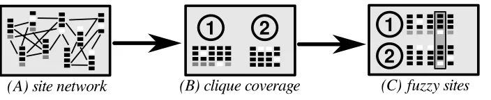
(A) site network

1

2

(B) clique coverage

1

2

(C) fuzzy sites

Figure 5

General workflow of the method for automatic correspondence pattern recognition.

Parsimony dictates that—when partitioning our alignment site graph—we should try to minimize the number of cliques to which the different nodes are assigned. This is theminimum clique cover problem(Bhasker and Samad 1991, page 2). The minimum clique cover problem is a well-known problem in graph theory and computer science, although it is usually more prominently discussed in the form of its inverse problem,12 thegraph coloring problem. In the graph coloring problem, one tries to assign all those nodes in a graph to different clusters (i.e., to “color” them in different colors) which are directly connected (Hetland 2010, page 276). While the problem is generally known to beNP-hard(Hetland 2010, page 276), fast approximate solutions like the Welsh-Powell algorithm (Welsh and Powell 1967) are available. Using approximate solutions seems to be appropriate for the task of correspondence pattern recognition, given that we do not (yet) have formal linguistic criteria to favor one clique cover over another.13

4. An Automatic Method for Correspondence Pattern Recognition

The method for automatic correspondence pattern recognition requires that the data be coded for cognacy, and that all cognate sets be phonetically aligned. Thanks to recently proposed algorithms, these tasks can be carried out automatically,14 _{but to guarantee} reliable results, it is useful to provide manually annotated data, or to manually correct data that was automatically analyzed in a first step.15

The general workflow of the method consists of three basic steps (see Figure 5). In a first step, the alignments in the data are used to construct analignment site network in which edges are drawn between compatible sites (A). The alignment sites are then partitioned into distinct non-overlapping subsets using an approximate algorithm for the minimum clique cover problem (B). In the final step (C), alternate correspondence sets are considered for each individual alignment site. Any existing partitions with which the site is compatible are added as potential correspondents. In the following sections, I will provide more detailed explanations on the different stages.

12 The inverse problem of a given problem in graph theory provides a solution to the original problem for a graph in which the original edges are deleted and nodes formerly unconnected are connected.

13 We should furthermore bear in mind that an optimal resolution of sound correspondence patterns for linguistic purposes would additionally allow for uncertainty when it comes to assigning a given alignment site to a given sound correspondence pattern. If we decided, for example, that the pattern C in Figure 1 could by no means cluster with E and F, this may well be premature before we have figured out whether the two patterns (u-u-u-uvs.u-u-u-au) arecomplementaryand what phonetic environments explain their complementarity.

14 For automatic cognate detection, compare for example List (2014), List, Greenhill, and Gray (2017), Arnaud, Beck, and Kondrak (2017), and Jäger, List, and Sofroniev (2017), and for automatic phonetic alignment, compare Proki´c, Wieling, and Nerbonne (2009) and List (2014).

Table 3

Input format with the basic values needed to apply the method for automatic correspondence pattern recognition.

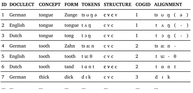
ID DOCULECT CONCEPT FORM TOKENS STRUCTURE COGID ALIGNMENT

1 German tongue Zunge ts ʊ ŋ ə c v c 1 ts ʊ ŋ ( ə )

2 English tongue tongue t ʌ ŋ c v c 1 t ʌ ŋ ( - )

3 Dutch tongue tong t ɔ ŋ c v c 1 t ɔ ŋ ( - )

4 German tooth Zahn ts aːn c v c 2 ts aː n

-5 English tooth tooth t uː θ c v c 2 t uː - θ

6 Dutch tooth tand tɑn t c v c 2 t ɑ n t

7 German thick dick d ɪk c v c 3 d ɪ k

... ... ... ... ... ... ... ...

c v c v

c v c c

4.1 Implementation, Input Format, and Output Format

The method has been implemented as a Python package that can be used as a plug-in for the Lplug-ingPy library for quantitative tasks plug-in historical lplug-inguistics (List, Greenhill, and Forkel 2017). The supplementary material offers precise instructions on how the software package can be installed and how the experiments can be replicated.

The input format for the method described here generally follows the input format employed by LingPy. In general, this format is a tab-separated text file with the first row being reserved for the header, and the first column reserved for a unique numer-ical identifier. The header specifies the entry types in the data. Table 3 provides an example of the minimal data that needs to be provided to our method for automatic correspondence pattern recognition. In addition to the generally needed information on the identifier of each word (ID), on the language (DOCULECT), the concept or elicita-tion gloss (CONCEPT), the (not necessarily required) orthographic form (FORM), and the phonetic transcription provided in space-segmented form (TOKENS), the method requires information on the type of sound (consonant or vowel, STRUCTURE),16 _the cognate set (COGID), and the alignment (ALIGNMENT).

The method offers different output formats, ranging from the LingPy wordlist format in which additional columns added to the original wordlist provide information on the inferred patterns, or in the form of tab-separated text files, in which the patterns are explicitly listed. The wordlist output can also be directly inspected in the EDICTOR tool, allowing for a convenient manual inspection of the inferred patterns.

4.2 Detailed Description of the Algorithm

As mentioned above, the method for correspondence pattern recognition consists of three stages. It starts with the reconstruction of an alignment site network in which each node represents a unique alignment site, and links between alignment sites are drawn if the sites are compatible, following the criterion for site compatibility outlined in Section 3 (A). It then uses a greedy algorithm to compute an approximate minimal clique cover of the network (B). All partitions proposed in stage (B) qualify as potentially valid correspondence patterns of our data. But the individual alignment sites in a given data set may as well be compatible with more than one correspondence pattern.17 _For this reason, the method iterates again over all alignment sites in the data, checking whether each is compatible with any other existing partition. This procedure assigns each alignment site to at least one but potentially more different sound correspondence patterns (C).18

The clique cover algorithm (A) is an inverse version of the Welsh-Powell algorithm for graph coloring (Welsh and Powell 1967). It starts withkcliques of size 1, which are sorted in increasing order by the amount of missing data they contain. The algorithm then picks the first pattern and compares it with the set of all other patterns. If this first pattern is compatible with one of the other patterns, the two patterns will be merged into a new pattern that is then further compared with the remaining ones. After the iteration, the first pattern is added to the set of results, and the same procedure is repeated with the remaining patterns that have not yet been merged and remain in the queue until no patterns are left.

Since alignment sites may suffer from missing data, their assignment to particular correspondence patterns is not always unambiguous. The example alignment from Fig-ure 1, for example, would yield two general correspondence patterns, namelyu-u-u-au

versusu-u-u-u. While the assignment of alignment sites A and C in the figure would be unambiguous, sites E and F could be assigned to either partition, since they are missing the disambiguating data. In order to reflect the fuzziness of the partition assignment, the method therefore requires an additional step. In addition to the partition from stage (B), alternative partitions are found for E and F during stage (C). The patterns, to which a given alignment site is assigned, can further be ranked by counting the total amount of alignment sites with which they are compatible, thus allowing us to prefer only those site-to-pattern assignments that have a reasonable number of examples.

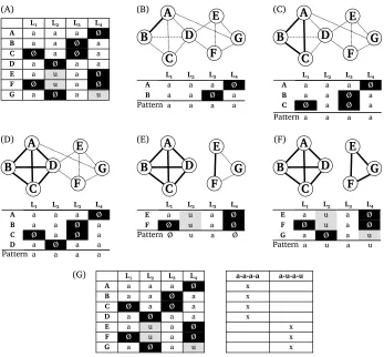
Figure 6 gives an artificial example that illustrates how the basic method infers the clique cover. Starting from the data in (A), the method assembles patterns A and B in (B) and computes their pattern, thereby retaining the non-missing data for each language in the pattern as the representative value. Having added C and D in this fashion in steps (C) and (D), the remaining three alignment sites, E–G, are merged to form a new partition, accordingly, in steps (E) and (F). Step (G) reflects the reassignment of individual alignment sites to the previously inferred patterns. In this example, all sites are only assigned to one pattern, but it is possible, depending on the amount of missing data, that one site can be assigned to more than one pattern.

17 Compare, for example, site E in Figure 1, which is both compatible with the patternu-u-u-ureflected by the site A, and the patternu-u-u-au, reflected by site B.

A

B

D

C

E

F

G

A

B

D

C

E

F

G

A

B

D

C

E

F

G

A

B

D

C

E

F

G

A

B

D

C

E

F

G

L₁ L₂ L₃ L₄

A a a a Ø

B a a Ø a

C Ø a Ø a

D a Ø a a

E a u a Ø

F Ø u a Ø

G a Ø a u

L₁ L₂ L₃ L₄

A a a a Ø

B a a Ø a

Øa a Øa a Pattern

L₁ L₂ L₃ L₄

A a a a Ø

B a a Ø a

Øa a Øa a Pattern

C Ø a Ø a

L₁ L₂ L₃ L₄

A a a a Ø

B a a Ø a

Øa a Øa a Pattern

C Ø a Ø a

D a Ø a a

L₁ L₂ L₃ L₄ Ø

ØØ u Øa Ø Pattern

E a u a Ø

F Ø u a Ø

L₁ L₂ L₃ L₄ Ø

Øa u Øa u Pattern

E a u a Ø

F Ø u a Ø

G a Ø a u

(A) (B) (C)

(D) (E) (F)

L₁ L₂ L₃ L₄ a-a-a-a a-u-a-u

A a a a Ø x

B a a Ø a x

C Ø a Ø a x

D a Ø a a x

E a u a Ø x

F Ø u a Ø x

G a Ø a u x

(G)

Figure 6

Example for the basic method to compute the clique cover of the data. (A) shows all alignment sites in the data. (B–D) show how the algorithm selects potential edges step by step in order to arrive at a first larger clique cover. (E–F) show how the second cover is inferred. In each step during which one new alignment site is added to a given pattern, the pattern is updated, filling empty spots. While there are two missing data points in (E), where only alignment sites E and F are merged, these are filled after adding G. (G) shows how patterns are reassigned to individual alignment sites.

It is important to note that the originally selected pattern may change during the merge procedure, since missing spots can be filled by merging the pattern with a new alignment site (as also shown in Figure 6). For this reason, it is possible that this procedure, when only carried out one time, may not result in a true clique cover (in which all compatible alignment sites are merged). For this reason, at the end of the iteration, the algorithm checks if patterns exist that could be further combined, and repeats the procedure with the existing patterns until the resulting partitioning represents a true clique cover.

Pseudocode is in Algorithm 1 for the core function of the method for correspon-dence pattern detection. In a worst-case scenario in which all alignment sites will be assigned to distinct correspondence patterns, the algorithm requiresPn_k=1 =n(n

Algorithm 1Main part of the correspondence pattern detection method in pseudocode.

1: functionCORRPATTERNS(almSites)

2: sort(almSites, sortKey:=countMissing); .sort the sites

3: patterns:=[]; .stores the patterns

4: whilelength(almSites)6=0do

5: first,rest:=almSites[0],almSites[1:]; .compare first site against rest

6: almSites:=[]; .fill with unmerged sites during for-loop

7: fori:=0;i<length(rest);i+ +do 8: ifcompatible(rest[i],first)then 9: first:=merge(first,rest[i]);

10: else

11: append(almSites,rest[i]);

12: end if

13: end for

14: append(patterns,first);

15: end while returnpatterns;

16: end function

however, this worst-case scenario is never reached, and the method converges rather fast.19

5. Testing the Method for Correspondence Pattern Recognition

The quantitative treatment of sound correspondence patterns presented in this study is novel. As a result, no expert-annotated data listing all observable correspondence patterns for a certain language family exhaustively is available.20_{and it is not possible} to compare the suitability of this novel approach with expert-annotated gold standards, as it is usually done in similar studies in computational historical linguistics.

The lack of suitable gold-standard data, however, does not mean that we cannot test the method for its suitability. Since the core service the method provides is to impute missing values in alignment sites resulting from cognate sets that are not reflected in all languages in a given data set, we can easily design tests in which we test the power of the method topredictthose missing values in controlled settings.

5.1 Data for Testing

Three different data sets were selected to test the method proposed in this study. The data sets were chosen with great care, since only a few of the many data sets offering manually coded cognate sets also provide the cognate sets in aligned form. Apart from the data by Hill and List (2017) on Burmish languages (original data based on Huáng 1992), Walworth (2018) on East Polynesian languages (original data based

19 This can easily be seen when assuming clique cover that includes all nodes in a given network: Here, the algorithm would need only one iteration, as it would consecutively merge each next node visited in the first iteration into the same partition.

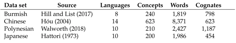
Table 4

Three test sets used in this study.

Data set Source Languages Concepts Words Cognates

Burmish Hill and List (2017) 8 240 1,819 798

Chinese Hóu (2004) 14 623 8,371 623

Polynesian Walworth (2018) 10 210 2,427 1,187

Japanese Hattori (1973) 10 200 1,986 454

on Greenhill, Blust, and Gray 2008), and Hattori (1973) on Japanese dialect (data in electronic form supplemented in List 2014), an additional data set of 14 Chinese varieties originally published by Hóu (2004) was specifically modified and manually aligned for this study. While the two former data sets are classical wordlists that are further coded for cognacy and alignments,21 _{the Chinese data is based on a collection of} 623 morphemes (reflected by a Chinese character each) whose pronunciation across the 14 dialects used in our sample was elicited by field workers. As a result, the amount of cognate sets with missing reflexes in this data set is extremely low.

An overview of the data sets, along with additional information regarding the data sources, the number of cognate sets, language varieties, and words in the data, is given in Table 4. Needless to say that all data sets are provided in the supplementary material accompanying this article.

5.2 General Characteristics

As a first illustrative test, the method was applied to the four data sets, and some basic statistics were calculated. These include the original number of alignment sites in the data, the number of patterns into which these sites were partitioned by the method, and the number of singleton patterns, that is, patterns that are reflected by only one alignment site in the data. By dividing the number of alignment sites assigned to non-unique patterns by the number of all sites, we can further determine the proportion of “regular” correspondence patterns in a given data set, assuming that a pattern is regular if it recurs in at least two different alignment sites.

The results of this analysis are summarized in Table 5. As we can see from this table, the number of correspondence patterns inferred by the algorithm is much lower than the number of alignment sites. This is, of course, not surprising, if we assume that the hypothesis that sound change is an overwhelmingly regular process holds. However, across the data sets, we can find rather large differences with respect to the amount of singleton patterns, that is, patterns reflecting only one alignment site. That an alignment site is not compatible with any other site in the data can have different reasons. First, there can be idiosyncratic sound changes, resulting, for example, from taboo, or from the assimilation of frequently used words. Second, there can be errors in the data, resulting from incorrectly assigned cognates, alignments, or undetected borrowings. It is also possible that the data sample is too small, and that additional samples could be found, but have not been included in the data.

Table 5

Basic statistics after applying the correspondence pattern recognition method to the four data sets.

Data set Align. Sites Corr. Patterns Singletons Reg. Patterns

Burmish 1,833 432 173 0.91

Chinese 2,891 1,341 966 0.67

Polynesian 1,863 243 64 0.97

Japanese 1,590 556 311 0.80

Table 6

Examples for idiosyncratic correspondence patterns in the Chinese dialects reflecting the major groups (Bˇeij¯ıng, S ¯uzh ¯ou, Chángsh¯a, Nánch¯ang, Méixiàn, Táoyuán, Guˇangzh ¯ou, Fúzh ¯ou, and Táibˇei [Mˇın dialect spoken in Táibˇei]).

When comparing the proportion of “regular” patterns that are reflected by at least two alignment sites in the data across the data sets, the Chinese data shows the lowest proportion, with only 67% of all alignment sites being assigned to patterns that recur in the data. Given the intertwined history of the Chinese dialects, in which language con-tact among the dialect varieties played an important role, it is not necessarily surprising that the data looks less regular in general: If languages borrow from each other, and borrowing is sporadic, rather than systematic, this will lead to an increase in irregular correspondence patterns and therefore impact on the regularity we can observe. As a manual inspection of the inferences reveals, the majority of the singleton alignment sites in the Chinese data could be assigned to one of the regular patterns if one of the reflexes would be ignored. Examples for these patterns are given in Table 6. On the other hand, we find some patterns that are largely irregular for specific reasons like taboo. An example is given in the same table with Chineseniˇao“bird” (pattern 679), which is reflected by nasal and dental initials across the Chinese dialects. As we know from older readings, the original reading had the initial[t], but it was later replaced by a nasal in some Chinese varieties to avoid homophony with the word for “penis,” which was most likely metaphorically shifted from “bird.”

with no more than 17 different sounds on average (compared to Chinese dialects with about 35 sounds), while many idiosyncratic patterns in the Japanese data result from morphological differences, which are difficult to handle in phonetic alignments.

5.3 Tests on Word Prediction

As mentioned briefly already in Section 1, correspondence patterns—once readily inferred—can provide hints regarding the potential pronunciation of missing cognates in an alignment. Since the method for correspondence pattern recognition imputes missing data in its core, it can also be used to predict how a given word should look in a given language if the reflex of the corresponding cognate set is missing. An example for the prediction of forms has been given above for the cognate set Dutchdorpand German Dorf. Since we know from Table 1 that the correspondence pattern ofd in Dutch and German usually points to Proto-Germanic *þ, we can propose that the English reflex (which is missing in Modern English, apart from place names) would start withth, if it was still preserved.22Since the method for correspondence pattern recognition assigns one or more correspondence patterns to each alignment site, even if the site has missing data for a certain number of languages, all that needs to be done in order to predict a missing entry is to look up the alignment pattern and check the value that is proposed for the given language variety.

The test on word prediction was designed as follows: from each of the data sets, a certain number of cognate sets was randomly deleted, and the resulting data was then analyzed with the help of the correspondence pattern recognition algorithm. In a second step, these inferred patterns were used to predict the cognate words which were deleted before. For the prediction, only the largest correspondence pattern was considered for the imputation, in order to avoid that multiple proposals for one sound could be made by the algorithm. For each data set, three different proportions of words to be deleted were tested (25%, 50%, and 75%).23For each proportion and data set, 1,000 trials were tested and the results were averaged. To assess the accuracy of a predicted word, the proportion of correctly predicted sounds in the given word was estimated and divided by the total length of the word. The individual accuracies of predicted words were then averaged by dividing the number of individual prediction scores by the number of predicted words for each trial.

The results of this experiment are given in Table 7. In general, we can note that the prediction experiment works very well across all data sets for wordlists reduced by 25% and 50% of their words appearing in cognate sets, while the accuracy of prediction drastically drops in all data sets when removing up to 75% of the data. The only exception is the Polynesian data set, where the difference in accuracy across the three experiments is only small, with a rather large standard deviation.

What may come as a surprise is that the reduction of the data by 25% and 50% does not seem to influence the accuracy of prediction in all data sets. On the contrary, in the Chinese and the Polynesian data sets, we find even slightly higher accuracy scores for the larger data reduction. At least in the Chinese data, the reason for this can be found in the large number of singleton patterns that deviate only in one reflex from regularly

22 We ignore deliberately in this context that the alternative of the correspondence in Dutch and German is a borrowing from Dutch, Frisian, or English to German.

Table 7

Results of the test on word prediction, based on 1,000 random samples for each subset of the data. The column Proportion reflects the different proportions of the data that was deleted during the experiments. Patterns refers to the average number of correspondence patterns inferred in each trial, and Reg. Patterns points to the proportion of alignment sites covered by patterns recurring at least twice.

Data set Proportion Patterns Reg. Patterns Accuracy Burmish 25% 231.68±6.86 0.94±0.01 0.59±0.02

50% 165.55±6.08 0.94±0.01 0.53±0.02 75% 99.33±5.71 0.89±0.02 0.37±0.03

Chinese 25% 1,040.62±11.88 0.81±0.01 0.69±0.01 50% 672.35±10.53 0.95±0.00 0.70±0.01 75% 373.23±7.67 0.97±0.00 0.64±0.01

Japanese 25% 399.82±10.04 0.89±0.01 0.64±0.01 50% 259.71±9.39 0.93±0.01 0.62±0.01 75% 142.65±7.35 0.92±0.01 0.52±0.02

Polynesian 25% 127.30±5.38 0.97±0.00 0.81±0.01 50% 89.10±5.51 0.97±0.01 0.82±0.01 75% 51.37±4.69 0.95±0.01 0.80±0.03

recurring patterns. If the data is reduced by 50%, the number of idiosyncratic patterns also drops, as we can see from the proportion of regularly recurring patterns given in the table. While these cover 95% of all alignment sites in the data set reduced by 50%, their proportion drops to 81% when being reduced by only 25%, and is (as we have seen in Table 5) even lower when analyzing the whole data set. If enough words are deleted from singleton patterns, like the ones shown in the examples in Table 6, the method for correspondence pattern recognition will assign them to the same clusters. As a result, the words whose pronunciation deviates will still be wrongly predicted, but the words that are not affected by individual sound changes will be predicted correctly, and since there are more regular words in the data, the overall prediction accuracy will increase.

When comparing the differences in the scores across the four data sets, we can also see that the overall “regularity” of the data, as measured by the number of patterns that recur more than one time, is not a good predictor of the success of the prediction quality. The Burmish data, for example, has rather high rates of pattern regularity, but performs worse in prediction than the other data sets. It is clear that the number of singleton patterns that only reflect one alignment site in a data set will have a direct impact on the word prediction quality, since only patterns that recur at least two times in the data can be used for prediction. But this is not the only factor influencing the prediction quality. Ambiguous alignment sites that can be assigned to more than one pattern may, for example, likewise produce erroneous predictions. For the time being, we cannot offer a full account of all the different factors that might influence prediction quality. More studies on different data sets will be needed to increase our knowledge in the future.

the method (for example, when carrying out field work or when searching for missing cognate sets), as it shows that we can reduce the amount of time spent on manual anno-tation substantially when annotating data sets for historical linguistics. Linguists could, for example, annotate half of their data manually and then use our method to impute potentially missing cognates in their data. If actual words that were not annotated in the first run turn out to have the same form as words predicted by our algorithm, this would be a very strong argument that they are really cognate. Another example would be guided field work for the purpose of historical language comparison. If insufficient amounts of data have been collected, scholars can use the prediction method to predict the most likely forms for certain cognate sets and use them to ease the elicitation of the relevant forms when asking new informants.

5.4 Examples

Table 8 gives some examples illustrating the scoring procedure and typical failures of the method, again illustrated for the Chinese data set.24_{In cognate set 687, we find one} correctly predicted form for Chángsh¯a, and one incorrectly predicted tone for the Jínán form. As we can see from the frequencies of alignment sites supporting the proposed pattern given in the column “Frequency” in the table, the inferred pattern clusters only two alignment sites. As a result, it is not surprising that a wrong tone is proposed. The wrong form for Mˇeixi¯an in cognate set 319 is due to a wrong clustering of the cognate set with the irregular cognate set 654, listed earlier in Table 6. Since the Mˇeixi¯an word was deleted in the experiment, the whole pattern is compatible with pattern # 73 in the table, which predicts that the Mˇeixi¯an form should start withth. In cognate set 518, we can see that the method fails to propose a valid sound for the form in W¯enzh ¯ou for the second and the third site in the alignment, given that these sites are assigned to singleton patterns (of one alignment site only) in which no sound for W¯enzh ¯ou could be imputed.

While the success or failure of the prediction experiments can help us to improve the method in the future, we can also illustrate how the analysis can aid in practical work on linguistic reconstruction. This example will again be based on the Chinese data, since it has the advantage of offering quick access to Middle-Chinese reconstructions. Because Middle Chinese is only partially reconstructed on the basis of historical lan-guage comparison, and mostly based on written sources, such as ancient rhyme books and rhyme tables (Baxter 1992), the reconstructions are not entirely dependent on the modern dialect readings, which is a great advantage for testing the consequences of the correspondence pattern analysis.

In Table 9, patterns inferred by the method for correspondence pattern recognition for a reduced number of dialects (one of each major subgroup) have been listed. The examples can all be reconstructed to a dental stop in Middle Chinese (*t, *th, or *d). If we inspect only reflexes of Middle Chinese *din the data, we can see that the initial consonant is reflected in seven different patterns in our data. Four of these patterns, however, occur only one time (# 719, # 1096, # 484, and # 654), as reflected in the column Cogn. (pointing to supportingcognate sets), and if we exclude the reflexes for Méixiàn

Table 8

Examples for the word prediction experiment for the Chinese data. The column Frequency lists the size of the inferred patterns for each position of the predicted word form. The score is calculated by dividing the number of correctly predicted sounds by the total number of sounds.

(# 719, # 654), Táibˇei (# 1096), and Nánch¯ang (# 484), respectively, we can assign # 719 and # 1096 to # 718 and # 484 and # 654 to # 73. In patterns # 718 and # 747, only Fúzh ¯ou shows a different reflex. Since we have forms that are homophones in Middle Chinese in both correspondence patterns ( in # 747 and in # 718 were both pronounced as *damin Middle Chinese), we cannot find a conditioning context that would explain this difference from the perspective of Middle Chinese alone. We know, however, that the Mˇin dialects (to which Fúzh ¯ou belongs) reflect features that are more archaic than Mid-dle Chinese. In this case, the difference between the patterns is regularly reflecting the difference between plain voiced and breathy voiced initials in the ancestor of the Mˇın dialects, with the latter going back to complex onsets in Old Chinese, the predecessor of all Chinese dialects (Baxter and Sagart 2014, page 171f). Furthermore, if we compare the patterns # 747 and # 73 directly, we can see that, although only Fúzh ¯ou has a direct reflex of the original voiced sound in Middle Chinese, we can still find its traces in the different correspondence patterns, since Bˇeij¯ıng and Guˇangzh ¯ou have contrastive outcomes in both patterns ([th]versus[t]). When inspecting the tones that are reconstructed for the different words in Middle Chinese, we can easily find a conditioning context where the reflexes differ. Thepíng(flat) tone category in Middle Chinese correlates with aspiration, while the other tone categories correlate with devoicing in the three dialects.25If we had no knowledge of Middle Chinese, it would be harder to understand that both patterns correspond to the same proto-sound, but once assembled in such a way, it would still be much easier for scholars to search for a conditioning context that allows them to assign the same proto-sound to the two patterns in questions.

The example shows that, as far as the Middle Chinese dental stops are concerned, we do not find explicit exceptions in our data, but can rather see that multiple corre-spondence patterns for the same proto-sound may easily evolve. We can also see that a careful alignment and cognate annotation is crucial for the success of the method, but

Table 9

Contrasting inferred correspondence patterns with Middle Chinese reconstructions (MC) and tone patterns (MC Tones: P: píng (flat), S: shˇang (rising), Q: qù (falling), R: rù (stop coda)) for representative dialects of the major groups (Bˇeij¯ıng, S ¯uzh ¯ou, Chángsh¯a, Nánch¯ang, Méixiàn, Táoyuán, Guˇangzh ¯ou, Fúzh ¯ou, Táibˇei).

even if the cognate judgments are fine, but the data are sparse, the method may propose erroneous groupings.

In contrast to manual work on linguistic reconstruction, where correspondence pat-terns are never regarded in the detail in which they are presented here, the method has the potential to drastically increase both the transparency and the quality of linguistic data sets, especially in combination with tools for cognate annotation, like EDICTOR, to which we added a convenient way to inspect inferred correspondence patterns interac-tively (see the example in Appendix A). Because linguists can run the new method on their data and then directly inspect the consequences by browsing all correspondence patterns conveniently in the EDICTOR, the method makes it a lot easier for linguists to come up with first reconstructions or to identify problems in the data.

6. Conclusion and Outlook

Supplementary Material

The supplementary material accompanying this article contains the code and all in-structions needed to repeat the experiments described in this article. The original package for correspondence pattern detection is publicly available from GitHub under https://github.com/lingpy/lingrex(Version 0.1.0). The package providing the sup-plementary material with results and instructions for running the code is also available via GitHub under https://github.com/lingpy/correspondence-pattern-paper (Version 1.1.1) and has been archived with Zenodo at https://doi.org/10.5281/ zenodo.1544949.

Appendix A: Inspecting Correspondence Patterns in EDICTOR

Acknowledgments

This research was funded by the DFG research fellowship grant 261553824 “Vertical and lateral aspects of Chinese dialect history” (2015–2016), and by the ERC Starting Grant 715618 “Computer-Assisted Language Comparison”

(http://calc.digling.org, 2017-2018). Originally, the approach presented here was inspired by a novel (so far still unpublished) biological technique presented to me by Eric Bapteste and Philippe Lopez, which later turned out to be completely different from the one presented here, as I misunderstood the original intention of the draft. This misunderstanding, which helped me to address a problem that had been following me for a long time, reflects how inspiring my collaboration with Eric and Philippe was. I am particularly indebted to Nathan W. Hill for supporting this project from the

beginning, by discussing the findings, the methods, and their potential improvement. I am also extremely thankful to Taraka Rama for commenting on many previous versions of this draft and the code, discussing details and recommending enhancements, as well as to Simon J. Greenhill for his support after I received the first reviews, and Mary Walworth for helping with data. Timotheus Bodt also deserves special thanks for being an early tester of the methods. In addition, many people provided helpful comments on an earlier version(s) of this article, including Adam Powell, David A. S. Moslehi, Eugen Hill, Juho Pystynen, Martin Kümmel, Rémy Viredaz, Tiago Tresoldi, and Yoram Meroz, to whom I would also like to express my gratitude.

References

Anttila, Raimo. 1972.An Introduction to Historical and Comparative Linguistics, Macmillan, New York.

Arnaud, Adam S., David Beck, and Grzegorz Kondrak. 2017. Identifying cognate sets across dictionaries of related languages. In Proceedings of the 2017 Conference on Empirical Methods in Natural Language Processing, pages 2509–2518, Association for Computational Linguistics.

Baxter, William H. 1992.A Handbook of Old Chinese Phonology. de Gruyter, Berlin. Baxter, William H., and Laurent Sagart. 2014.

Old Chinese. A New Reconstruction. Oxford University Press, Oxford.

Beekes, Robert S. P. 1995.Comparative Indo-European Linguistics. An Introduction. John Benjamins, Amsterdam and Philadelphia.

Bhasker, J., and Tariq Samad. 1991. The clique-partitioning problem.Computers & Mathematics with Applications, 22(6):1–11. Blust, Robert. 1990. Patterns of sound

change in the Austronesian languages. In Philip Baldi, editor,Linguistic Change and Reconstruction Methodology. Mouton de Gruyter, Berlin; New York, pages 231–270.

Brown, Cecil H., David Beck, Grzegorz Kondrak, James K. Watters, and Søren Wichmann. 2011. Totozoquean.

International Journal of American Linguistics, 77(3):323–372.

Brown, Cecil H., Eric W. Holman, and Søren Wichmann. 2013. Sound correspondences in the world’s languages.Language, 89(1):4–29.

Campbell, Lyle, and William John Poser. 2008.Language Classification: History and Method. Cambridge University Press, Cambridge.

Clackson, James. 2007.Indo-European Linguistics. Cambridge University Press, Cambridge.

Covington, Michael A. 1996. An algorithm to align words for historical comparison. Computational Linguistics, 22(4):481–496. Dixon, R. B., and A. L. Kroeber. 1919.

Linguistic Families of California. University of California Press, Berkeley.

Dybo, Anna, and George S. Starostin. 2008. In defense of the comparative method, or the end of the Vovin controversy. In I. S. Smirnov, editor,Aspekty komparativistiki, Volume 3. RGGU, Moscow, pages 119–258. Fox, Anthony. 1995.Linguistic Reconstruction.

Oxford University Press, Oxford. Greenhill, Simon J., Robert Blust, and

Russell D. Gray. 2008. The Austronesian Basic Vocabulary Database: From bioinformatics to lexomics.Evolutionary Bioinformatics, 4271–283.

Grimes, Joseph E., and Frederick B. Agard. 1959. Linguistic divergence in romance. Language, 35(4):598–604.

Guy, Jacques B. M. 1994. An algorithm for identifying cognates in bilingual wordlists and its applicability to machine

translation.Journal of Quantitative Linguistics, 1(1):35–42.

Hattori, Shir ¯o. 1973. Japanese dialects. In Henry M. Hoenigswald and Robert H. Langacre, editors.Diachronic, Areal and Typological Linguistics,Number 11 in Current Trends in Linguistics.Mouton, The Hague and Paris, pages 368–400.

Hill, Nathan W., and Johann-Mattis List. 2017. Challenges of annotation and analysis in computer-assisted language comparison: A case study on Burmish languages.Yearbook of the Pozna ´n Linguistic Meeting, 3(1):47–76.

Hoenigswald, Henry Max. 1960.Language Change and Linguistic Reconstruction, 4. aufl. 1966 edition. The University of Chicago Press, Chicago.

Holton, Gary, Marian Klamer, František Kratochvíl, Laura C. Robinson, and Antoinette Schapper. 2012. The historical relations of the Papuan languages of Alor and Pantar.Oceanic Linguistics,

51(1):86–122.

Hóu, J¯ıng¯ı. 2004.Xiàndài Hàny ˇu f¯angyán y¯ınkù [Phonological Database of Chinese Dialects], Shànghˇai Jiàoyù, Shànghˇai.

Huáng, Bùfán. 1992.Zàngmiˇan y ˇuzú y ˇuyán cíhuì, Zh ¯ongy¯ang Mínzú Dàxué [Central Institute of Minorities], Beij¯ıng.

Jacques, Guillaume. 2017. A reconstruction of Proto-Kiranti verb roots.Folia Linguistica Historica, 38(1):177–215.

Jäger, Gerhard, Johann-Mattis List, and Pavel Sofroniev. 2017. Using support vector machines and state-of-the-art algorithms for phonetic alignment to identify cognates in multi-lingual wordlists. InProceedings of the 15th Conference of the European Chapter of the Association for Computational Linguistics. Long Papers. pages 1204–1215.

Kay, Martin. 1964.The Logic of Cognate Recognition in Historical Linguistics. The RAND Corporation, Santa Monica. Kondrak, Grzegorz. 2000. A new algorithm

for the alignment of phonetic sequences. InProceedings of the 1st North American Chapter of the Association for Computational Linguistics Conference, pages 288–295. Kondrak, Grzegorz. 2002. Determining recurrent sound correspondences by inducing translation models. InNineteenth International Conference on Computational Linguistics, pages 488–494, Taipei. Kondrak, Grzegorz. 2003. Identifying

complex sound correspondences in bilingual wordlists. Alexander Gelbukh, editor.Computational Linguistics and Intelligent Text Processing. Springer, Berlin, pages 432–443.

Kondrak, Grzegorz. 2009. Identification of cognates and recurrent sound correspondences in word lists.Traitement Automatique des Langues, 50(2):201–235. Kroonen, Guus. 2013.Etymological Dictionary

of Proto-Germanic.Number 11 inLeiden Indo-European Etymological Dictionary Series. Brill, Leiden and Boston.

List, Johann-Mattis. 2012. LexStat. Automatic detection of cognates in multilingual wordlists. InProceedings of the EACL 2012 Joint Workshop of Visualization of Linguistic Patterns and Uncovering Language History from Multilingual Resources, pages 117–125, Stroudsburg.

List, Johann-Mattis. 2014.Sequence Comparison in Historical Linguistics. Düsseldorf University Press, Düsseldorf.

List, Johann-Mattis. 2016. Computer-assisted language comparison: Reconciling computational and classical approaches in historical linguistics. Technical Report, Max Planck Institute for the Science of Human History, Jena.

List, Johann-Mattis. 2017. A web-based interactive tool for creating, inspecting, editing, and publishing etymological datasets. InProceedings of the 15th Conference of the European Chapter of the Association for Computational Linguistics. System Demonstrations. pages 9–12, Association for Computational Linguistics, Valencia.

List, Johann-Mattis, Simon Greenhill, and Robert Forkel. 2017.LingPy. A Python Library for Quantitative Tasks in Historical Linguistics. Max Planck Institute for the Science of Human History, Jena.

List, Johann-Mattis, Simon J. Greenhill, and Russell D. Gray. 2017. The potential of automatic word comparison for historical linguistics.PLOS ONE, 12(1):1–18. McMahon, April, and Robert McMahon.

2005.Language Classification by Numbers. Oxford University Press, Oxford. Meier-Brügger, Michael. 2002.

Indogermanische Sprachwissenschaft, 8th edition. de Gruyter, Berlin and New York. Meillet, Antoine. 1908.Les dialectes

Indo-Européens, Librairie Ancienne Honoré Champion, Paris.

Meillet, Antoine. 1954.La méthode comparative en linguistique historique, reprint edition. Honoré Champion, Paris.

Needleman, Saul B., and Christan D. Wunsch. 1970. A gene method applicable to the search for similarities in the amino acid sequence of two proteins.Journal of Molecular Biology, 48:443–453.

Newman, M. E. J. 2010.Networks. An Introduction. Oxford University Press, Oxford.