Synchronous Context Free Grammars and Optimal Parsing Strategies

and Optimal Parsing Strategies

Daniel Gildea

Giorgio Satta

The complexity of parsing with synchronous context-free grammars is polynomial in the sentence length for a fixed grammar, but the degree of the polynomial depends on the grammar. Specifi-cally, the degree depends on the length of rules, the permutations represented by the rules, and the parsing strategy adopted to decompose the recognition of a rule into smaller steps. We address the problem of finding the best parsing strategy for a rule, in terms of space and time complexity. We show that it is NP-hard to find the binary strategy with the lowest space complexity. We also show that any algorithm for finding the strategy with the lowest time complexity would imply improved approximation algorithms for finding the treewidth of general graphs.

1. Introduction

Synchronous context-free grammars (SCFGs) generalize context-free grammars (CFGs) to generate two strings simultaneously. The formalism dates from the early days of automata theory; it was developed under the name syntax-direct translation sche-mata to model compilers for programming languages (Lewis and Stearns 1968; Aho and Ullman 1969). SCFGs are widely used today to model the patterns of re-ordering between natural languages, and they form the basis of many state-of-the-art statistical machine translation systems (Chiang 2007).

Despite the fact that SCFGs are a very natural extension of CFGs, and that the parsing problem for CFGs is rather well understood nowadays, our knowledge of the parsing problem for SCFGs is quite limited, with many questions still left unanswered. In this article we tackle one of these open problems.

Unlike CFGs, SCFGs do not admit any canonical form in which rules are bounded in length (Aho and Ullman 1972), as for instance in the well-known Chomsky normal form for CFGs. A consequence of this fact is that the computational complexity of parsing with SCFG depends on the grammar. More precisely, for a fixed SCFG, parsing is polynomial in the length of the string. The degree of the polynomial depends on the

∗Computer Science Department, University of Rochester, Rochester NY 14627. E-mail:gildea@cs.rochester.edu.

∗∗Dipartimento di Ingegneria dell’Informazione, Universit`a di Padova, Via Gradenigo 6/A, 35131 Padova, Italy. E-mail:satta@dei.unipd.it.

Submission received: 28 July 2015; revised version received: 4 February 2016; accepted for publication: 8 February 2016.

length of the grammar’s rules, the re-ordering patterns represented by these rules, as well as the strategy used to parse each rule. The complexity of finding the best parsing strategy for a fixed SCFG rule has remained open. This article shows that it is NP-hard to find the binary parsing strategy having the lowest space complexity. We also consider the problem of finding the parsing strategy with the lowest time complexity, and we show that it would require progress on long-standing open problems in graph theory either to find a polynomial algorithm or to show NP-hardness.

The parsing complexity of SCFG rules increases with the increase of the number of nonterminals in the rule itself. Practical machine translation systems usually confine themselves to binary rules, that is, rules having no more than two right-hand side nonterminals, because of the complexity issues and because binary rules seem to be adequate empirically (Huang et al. 2009). Longer rules are of theoretical interest because of the naturalness and generality of the SCFG formalism. Longer rules may also be of practical interest as machine translation systems improve.

For a fixed SCFG, complexity can be reduced byfactoringthe parsing of a grammar rule into a sequence of smaller steps, which we refer to as aparsing strategy. Each step of a parsing strategy collects nonterminals from the right-hand side of an SCFG rule into a subset, indicating that a portion of the SCFG rule has been matched to a subsequence of the two input strings, as we explain precisely in Section 2. A parsing strategy is binary if it combines two subsets of nonterminals at each step to create a new subset. We consider the two problems of finding the binary parsing strategy with optimal time and space complexity. For time complexity, there is no benefit to considering parsing strategies that combine more than two subsets at a time. For space complexity, the lowest complexity can be achieved with no factorization whatsoever; however, con-sidering binary parsing strategies can provide an important trade-off between time and space complexity. Our results generalize those of Crescenzi et al. (2015), who show NP-completeness for decision problems related to both time and space complexity forlinear

parsing strategies, which are defined to be strategies that add one nonterminal at a time. Our approach constructs a graph from the permutation of nonterminals in a given SCFG rule, and relates the parsing problem to properties of the graph. Our results for space complexity are based on the graph theoretic concept of carving width, whose decision problem is NP-complete for general graphs. Section 3 relates the space com-plexity of the SCFG parsing problem to the carving width of a graph constructed from the SCFG rule. In Section 4, we show that any polynomial time algorithm for optimizing the space complexity of binary SCFG parsing strategies would imply a polynomial time algorithm for carving width of general graphs. Our results for time complexity are based on the graph theoretic concept oftreewidth. In Section 5, we show that any polynomial time algorithm for the decision problem of the time complexity of binary SCFG strategies would imply a polynomial time constant–factor approximation algo-rithm for the treewidth of general graphs. In the other direction, NP-completeness of the decision problem of the time complexity for SCFG would imply the NP-completeness of treewidth of general graphs of degree six. These are both long-standing open problems in graph theory.

2. Synchronous Context-Free Grammars and Parsing Strategies

summarize the adopted notation. Throughout this article, for any positive integernwe write [n] to denote the set{1,. . .,n}.

2.1 Synchronous Context-Free Grammars

As usual, a CFG has a finite set of rules having the general formA→α, where Ais a nonterminal symbol to be rewritten andα is a string of nonterminal and terminal symbols. Asynchronous context-free grammaris a rewriting system based on a finite set of so-called synchronous rules. Each synchronous rule has the general form [A1→ α₁, A2→α2], whereA1 →α1 andA2 →α2 are CFG rules. By convention, we refer to A1 →α1andA2→α2as the Chinese and English components of the synchronous rule, respectively. Furthermore,α₁,α₂ must be synchronous strings. This means that there exists a bijection between the occurrences of nonterminals inα₁and the occurrences of nonterminals in α₂, and that this bijection is explicitly provided by the synchronous rule. Nonterminal occurrences that correspond under the given bijection are called

linkednonterminal occurrences, or just linked nonterminals when no ambiguity arises. We assume that linked nonterminals always have the same label.

As a simple example, consider the synchronous rule

[A→aA1 bB2

d, A→bB2 cA1

]

whereA,Bare nonterminal symbols anda,b,c,d are terminal symbols. We have indi-cated the bijection associated with the synchronous rule by annotating the nonterminal occurrences with natural numbers, with the intended meaning that linked nonterminals get the same number. We refer to this number as a nonterminal’sindex.

The bijection associated with a synchronous rule plays a major role in the derivation of a pair of strings by the SCFG. In fact, in an SCFG we can only apply a synchronous rule to linked nonterminals. To illustrate this, we use our running example and consider the synchronous strings [A1

, A1

]. We can construct a derivation by applying our synchronous rule to the linked nonterminals, written

[A1 , A1

]⇒[aA2 bB3

d, bB3 cA2

]

Note that we have renamed the indices in the synchronous rule to make them disjoint from the indices already in use in the synchronous string to be rewritten. Although this is unnecessary in this first derivation step, this strategy will always be adopted to avoid conflicts in more complex derivations. We can move on with our derivation by applying once more our synchronous rule to rewrite the linkedAnonterminals, obtaining

[A1 , A1

]⇒[aA2 bB3

d, bB3 cA2

]⇒[aaA4 bB5

dbB3 d, bB3

cbB5 cA4

]

In this derivation, the renaming of the indices is crucial to avoid conflicts.

LetSbe a special nonterminal of our SCFG, which we call the starting nonterminal. Using our notion of derivation, one can start from [S1

, S1

Example 1

Consider the following list of synchronous rules, where symbolssiare rule labels to be

used later as references

s1 : [S→A 1

B2

, S→B2 A1

] s2 : [A→aA1b, A→bA1a] s3 : [A→ab, A→ba] , s4 : [B→cB1d, B→dB1c] s5 : [B→cd, B→dc]

What follows is a valid derivation of the SCFG, obtained by rewriting at each step the linked nonterminals with the Chinese component occurring at the left-most position in the sentential form

[S1 , S1

]⇒s1 _[A2_B3_,B3_A2_]

⇒s2 _[aA4_bB3_,B3_bA4_a]

⇒s2 _[aaA5_bbB3_,B3_bbA5_aa]

⇒s3 _[aaabbbB3_,B3_bbbaaa]

⇒s4 _[aaabbbcB6_d,dB6_cbbbaaa]

⇒s5 _{[aaabbbccdd,ddccbbbaaa]}

It is not difficult to see that the given SCFG provides the translation {[apbpcqdq, dqcqbpap]|p,q≥1}.

One can also associate SCFG derivations with parse trees, in a way very similar to what we do with CFG derivations. More precisely, an SCFG derivation is represented as a pair of parse trees, each generating one component in the derived string pair. Furthermore, linked nonterminals in the SCFG derivation are annotated in the parse trees to indicate the place of application of some synchronous rule.

Example 2

The SCFG derivation for string pair [aaabbbccdd,ddccbbbaaa] in Example (1) is associated with the following tree pair:

S1

A2 _B3

a _A4 _b

a _A5 _b

a b

c _B6 _d

c d

S1

B3 _A2

d _B6 _c

d c

b _A4 _a

b A5 a

One common view of SCFGs is that each synchronous rule implements a permuta-tion of the (occurrences of the) nonterminal symbols in the two rule components. More precisely, the nonterminals in the right-hand side of the Chinese rule component are re-used in the right-hand side of the English component, but with a different ordering, as defined by the bijection associated with the rule. This reordering is at the core of the translation schema implemented by the SCFG. We will often use the permutation view of a synchronous rule in later sections.

As already mentioned, we assume that linked nonterminals in a synchronous rule have the same label. In natural language processing applications, this is by far the most common assumption, but one might also drop this requirement. The results presented in this article do not rest on such a restriction.

2.2 Parsing Strategies

The recognition and the parsing problems for SCFGs are natural generalizations of the same problems defined for CFGs. Given an SCFG of interest, in the recognition problem one has to decide whether an input pair [u,v] can be generated. In addition, for the parsing problem one has to construct a parse forest, in some compact representation, with all tree pairs that the SCFG produces when generating [u,v]. When dynamic programming techniques are used, it turns out that recognition and parsing algorithms are closely related, since the elementary steps that are performed during recognition can be memoized and later used to construct the desired parse forest.

Despite the similarity between CFGs and SCFGs, it turns out that there is a consid-erable gap in the space and time complexity for recognition and parsing based on these two classes. More specifically, for a fixed CFG, we can solve the recognition problem in time cubic in the length of the input string, using standard dynamic programming techniques. In contrast, for a fixed SCFG we can still recognize the input pair [u,v] in polynomial time, but the degree of the polynomial depends on the specific structure of the synchronous rules of the grammar, and can be much larger than in the CFG case. A similar scenario also holds for the space complexity. The reason for this gap is informally explained in what follows.

In the investigation of the recognition problem for CFGs and SCFGs, a crucial notion is the one of parsing strategy. Recognition algorithms can be seen as sequences of elementary computational steps in which two parse trees that generate non-overlapping portions of the input are combined into a larger parse tree, according to the rules of the grammar. We call parsing strategy any general prescription indicating the ex-act order in which these elementary steps should be carried out. Generally speak-ing, parsing strategies represent the order in which each parsing tree of the input is constructed.

For the CFG case, let us consider the standard top–down chart parsing algorithm of Kay (1980). The algorithm adopts a parsing strategy that visits the nonterminals in the right-hand side of a rule one at a time and in a left-to-right order, combining the associated parse trees accordingly. Parse trees are then compacted into so-called chart edges, which record the two endpoints of the generated substring along with other grammar information. Chart parsing can be generalized to SCFGs. However, in the latter case parse trees no longer generate single substrings: They rather generate tuples with several substrings. This can be ascribed to the added component in synchronous rules and to the re-ordering of the nonterminals across the two components.

fan-out affects the number of stored edges for a given input string, and is directly connected to the space and time performance of the algorithm. A binary parsing strat-egy of fan-out ϕ has space complexity O(n2ϕ) and time complexity at most O(n3ϕ) wherenis the sentence length (Seki et al. 1991; Gildea 2010). If we adopt the appropriate parsing strategy, we can reduce the fan-out, resulting in asymptotic improvement in the space and time complexity of our algorithm. To illustrate this claim we discuss a simple example.

Example 3

Consider the synchronous rule

s: [A→B1

B2

B3

B4

B5

B6

B7

B8

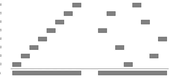
A→B5B7B3B1B8B6B2B4] (1)

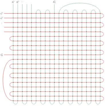
The permutation associated with this rule is schematically visualized in Figure 1. A naive parsing strategy for ruleswould be to collect the nonterminalsBk

one at a time and in ascending order ofk. For instance, at the first step we combineB1

and B2

, constructing a parse tree with fan-out 3, as seen from Figure 1. The worst case is attested when we construct the parse tree consisting of occurrencesB1

,. . .,B5

, which has a fan-out of 4.

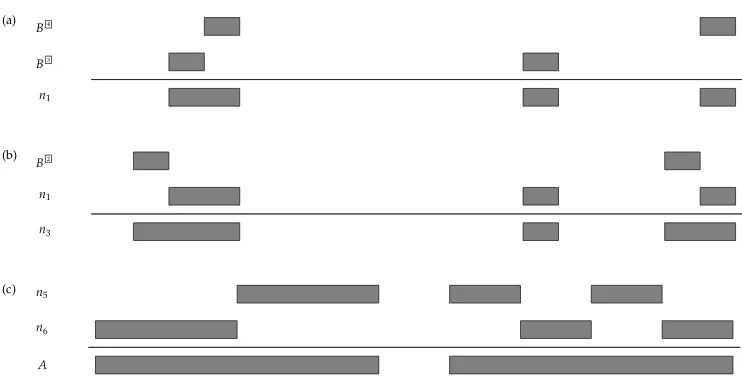
Alternatively, we could explore more flexible parsing strategies. An example is depicted in Figure 2, where each elementary step is represented as an internal node of a tree. This time, at the first step (node n1) we combine B3 and B4, as depicted in Figure 3a. At the second step (noden3), we combine the result of noden1 and B2, again constructing a parse tree with fan-out three, as depicted in Figure 3b, and so on. This strategy is non-linear, because it might combine parses containing more than one nonterminal occurrence each; see Figure 3c. From Figure 1 it is not difficult to check that at each nodenkthe constructed parse has fan-out bounded by 3. We therefore conclude

that our second strategy is more efficient than the left-to-right one.

B8

B7

B6

B5

B4

B3

B2

B1

A

Figure 1

n7

n5

B1

n3

B2

n1

B3 B4

n6

B5

n4

B6

n2

B7 B8 Figure 2

A bidirectional parsing strategy for rulesof Equation (1).

This example shows that the maximum fan-out needed to parse a synchronous rule depends on the adopted parsing strategy. In order to optimize the computational resources of a parsing algorithm, we need to search for a parsing strategy that minimizes the maximum fan-out of the intermediate parse trees. The problem that we investigate in this article is therefore the one of finding optimal parsing strategies for synchronous rules, where in this context optimal means with a value of the maximal fan-out as small as possible.

2.3 Fan-out and Parsing Optimization

In this section we provide a mathematical definition for the concepts that we have informally introduced in the previous section. We need to do so in order to be able to precisely define the computational problem that is investigated in this article.

(a)

B4

B3

n1

(b)

B2

n1

n3

(c) n5

n6

A

Figure 3

Assume a synchronous context-free ruleswithr≥2 linked nonterminals. We need to address occurrences of nonterminal symbols within s. We writeh1,ii to represent theith occurrence (from left to right) in the right-hand side of the Chinese component ofs. Similarly,h2,iirepresents theith occurrence in the right-hand side of the English component ofs. Each pairhh,ii,h∈[2] andi∈[r], is called anoccurrence.

We assume without loss of generality that the nonterminals of the Chinese compo-nent are indexed sequentially. That is, the index ofh1,iiisi. Letπbe the permutation over set [r] implemented by s, meaning thath2,ii is annotated with index π(i), and therefore is co-indexed with h1,π(i)i. As an example, in rule (1) we have r=8 and π(1)=5,π(2)=7,π(3)=3, etc. Under this convention, each pair (h1,π(i)i,h2,ii) and, equivalently, each pair (h1,ii,h2,π−1_{(i)i),i∈[r] is called alinked pair.}

Aparsing strategyforsis a rooted, binary treeτ_swithrleaves, where each leaf is a linked pair (h1,π(i)i,h2,ii). As already explained, the intended meaning is that each internal node ofτ_srepresents the operation of combining the linked pairs below the left node with the linked pairs below the right node. These operations must be performed in a bottom–up fashion.

Letnbe an internal node ofτ_s, and letτ_nbe the subtree ofτ_srooted atn. We write y(n) to denote the set of all occurrenceshh,iiappearing in the linked pair of some leaf ofτ_n. We say that occurrencehh,ii ∈y(n) is aright boundaryofnifi=ror ifi<rand

hh,i+1i 6∈y(n). Symmetrically, we say that hh,ii ∈y(n) is a left boundaryif i=1 or if i>1 andhh,i−1i 6∈y(n). Note that the occurrencesh1, 1iand h2, 1iare always left boundaries, andh1,riandh2,riare always right boundaries. We letbd(n) be the total number of right and left boundaries iny(n).

Intuitively, the number of boundaries iny(n) provides the number of endpoints of the substrings in the rule components ofsthat are spanned by the occurrences iny(n). Dividing this total number by two provides the number of substrings spanned by the occurrences iny(n). We therefore define thefan-outat nodenas

fo(n)=1

2bd(n) (2)

As discussed in Section 2.2, the largest fan-out over all internal nodes of a parsing strategy provides space and time bounds for a dynamic programming parsing algo-rithm adopting that strategy. Given an input synchronous rules, we wish to find the parsing strategy that minimizes quantity

min

τ maxn fo(n) (3)

whereτranges over all possible parsing strategies fors, andnranges over all possible nodes ofτ. One of the two main results in this article is that this optimization problem is NP-hard.

3. Cyclic Permutation Multigraphs and Carving Width

In this section, we relate the fan-out of parsing strategies for an SCFG rule to the properties of a specific graph derived from the rule’s permutation.

set of vertices and E is a set of edges, with each edge consisting of an unordered pair of vertices. A multigraph is a graph that uses a multiset of edges. This means that a multigraph can have several occurrences of an edge impinging on a pair of vertices.

A cyclic permutation multigraph is a multigraph G=(V,A]B) such that both PA=(V,A) and PB=(V,B) are Hamiltonian cycles, that is, cycles that visit all the

vertices inV exactly once. In the following, the edges inAwill be calledredand the edges inBwill be calledgreen. Our definition is based on the permutation multigraphs of Crescenzi et al. (2015), which differ in that they consist of two acyclic Hamiltonian paths.

In this article, we use cyclic permutation multigraphs to encode synchronous rules. Letsbe a synchronous rule withr≥2 linked pairs. Let also (h1, 0i,h2, 0i) be a special linked pair representing the left-hand side nonterminal ofs. We construct the cyclic permutation multigraphMs, representings, as follows. The linked pairs (h1,π(i)i,h2,ii),

i∈[r], along with (h1, 0i,h2, 0i), form the vertices of Ms. The red cycle of Ms begins

with (h1, 0i,h2, 0i), then follows the order in which nonterminals occur in the Chinese component ofs, and finally returns to (h1, 0i,h2, 0i). Similarly, the green cycle of Ms

begins and ends with (h1, 0i,h2, 0i), and follows the order in which nonterminals occur in the English component.

In the other direction, given any cyclic permutation multigraph, we can derive a corresponding SCFG rule by, first, choosing an arbitrary vertex as representing the left-hand side nonterminal, and then following the red cycle to obtain the sequence of Chinese nonterminals, and finally following the green cycle to obtain the sequence of English nonterminals.

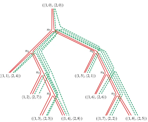
Example 4

Consider the SCFG rule s of Equation (1) in Example (3). Figure 4 shows the cyclic permutation multigraph associated withs. The red path starts at (h1, 0i,h2, 0i), followed by the vertices in the order of the Chinese nonterminals of the rule, that is, (h1, 1i,h2, 4i), (h1, 2i,h2, 7i), (h1, 3i,h2, 3i),. . ., (h1, 8i,h2, 5i). The green path starts at (h1, 0i,h2, 0i), followed by the vertices in the order of the English nonterminals, that is, (h1, 5i,h2, 1i), (h1, 7i,h2, 2i), (h1, 3i,h2, 3i),. . ., (h1, 4i,h2, 8i).

An important property of Ms is that every edge connects two linked pairs that

share a boundary in either the Chinese component of the rule (red edge) or in the English component (green edge). Note that, as a special case, we consider the linked pair (h1, 0i,h2, 0i) as sharing two left boundaries with the linked pairs (h1, 1i,h2,π−1(1)i)

(h1, 1i,h2, 4i) h1, 2i,h2, 7i) (h1, 3i,h2, 3i) (h1, 4i,h2, 8i) (h1, 5i,h2, 1i) (h1, 6i,h2, 6i) (h1, 7i,h2, 2i) (h1, 8i,h2, 5i) (h1, 0i,h2, 0i)

Figure 4

and (h1,π(1)i,h2, 1i), and as sharing two right boundaries with the linked pairs (h1,ri,h2,π−1(r)i) and (h1,π(r)i,h2,ri).

Consider any setSof linked pairs fromMssuch that (h1, 0i,h2, 0i)6∈S. LetSbe the

complement set ofS, that is,Sis the set of linked pairs fromMsnot inS. It is not difficult

to see that the multiset of edges connectingSandScorresponds to the set of boundaries of any parse tree associated with the linked pairs inS. We can apply this property to parsing strategies, which we have previously defined as rooted binary trees, in order to count the boundaries that are open after completing some parsing step represented by an internal noden, which we have defined asbd(n). Consider for instance the parsing strategy shown in Figure 2, and consider the internal noden3. At this node we have collected nonterminalsB2

,B3

, andB4

, and we havebd(n3)=6. If we consider the set Swith the corresponding linked pairs (h1, 2i,h2, 7i), (h1, 3i,h2, 3i), and (h1, 4i,h2, 8i), we can see that the number of edges of the multigraph that connectS withS is six, that is, exactly the value ofbd(n3). In order to express these observations in a mathematical way, we need to introduce the notions of tree layout, width, and carving width, which we borrow from graph theory.

Atree layout T of a graph Gis an undirected binary branching tree having one vertex ofGat each leaf. To avoid confusion, in what follows we use the termnodewhen referring to vertices of layout trees and we use the termarcwhen referring to edges of layout trees. Edges ofGare routed along the arcs ofT. A simple example is provided in Figure 5, showing a graphGand a tree layoutTofG.

Informally, the width of an arc ofTis the number of edges fromGthat are routed through that arc. We define this notion more precisely in what follows. We start with some auxiliary notation. LetVbe the set of vertices ofGand letSbe any subset ofV. Theedge boundaryofSinV, written∂_V(S), is the set of edges ofGthat connect vertices inSand vertices in the complement setS=V\S. Letabe an arc in a tree layoutTofG, and letT1 andT2 be the two components of the graph obtained by removingafromT. Let alsoL(T1) be the subset ofVappearing at the leaves ofT1. ThewidthofainTis the number of edges inGthat cross betweenT1andT2:

wdG,T(a)=|∂V(L(T1))| (4)

The maximum width among all of the arcs ofTis thecarving widthofT. The carving width ofTin Figure 5 is 3. The carving width ofGis the minimum carving width over all possible tree layouts ofG:

wd(G)=min

T maxa wdG,T(a) (5)

Figure 5

Deciding whether the carving width of arbitrary graphs is less than or equal to a given integer is an NP-complete problem (Seymour and Thomas 1994). Throughout this article, we extend to multigraphs all of the discussed notions of tree layout, width, and carving width, in the obvious way. Because graphs are a subset of multigraphs, carving width of multigraphs is also an NP-complete problem.

We can now apply the notion of tree layout to parsing strategies for SCFG rules, and show an important property that relates the notions of fan-out (equivalently, boundary count) and carving width. Letsbe an SCFG rule withrlinked pairs. Recall that a parsing strategy forsis a rooted binary tree where each leaf node is a linked pair representing some nonterminal from the right-hand side ofs. We attach to the root of our parsing strategy an additional leaf node, representing the special linked pair (h1, 0i,h2, 0i). The resulting tree hasr+1 leaves, and can therefore be used as a tree layout for the cyclic permutation multigraphMs encoding s. Furthermore, each internal node of the tree

layout is associated with a parsing step.

Example 5

Consider the SCFG rulesin Equation (1) and the associated cyclic permutation multi-graph Ms shown in Figure 4. Consider also the parsing strategy τs for s shown in

Figure 2. By attaching the linked pair (h1, 0i,h2, 0i) to the root node ofτ_s, we can derive a tree layoutTforMs, which is shown in Figure 6. Observe that every linked pair (vertex)

ofMs, including the special linked pair (h1, 0i,h2, 0i), is placed at some leaf node ofT,

and the edges ofMs are routed along arcs ofT. Letabe an arc ofT and letn be the

node belowa, with respect to the root node. Observe how edges that are routed along a correspond to boundaries that are open at the associated step n of the parsing strategyτ_s.

(h1, 0i,h2, 0i)

n7

n5

n3

n1

n6

n4

n2 (h1, 1i,h2, 4i)

h1, 2i,h2, 7i)

(h1, 3i,h2, 3i) (h1, 4i,h2, 8i) (h1, 5i,h2, 1i)

(h1, 6i,h2, 6i)

(h1, 7i,h2, 2i) (h1, 8i,h2, 5i)

Figure 6

The next lemma summarizes the connection between carving width and fan-out.

Lemma 1

The minimum fan-out of any parsing strategy of an SCFG rulesis half of the carving width of the cyclic permutation multigraph constructed froms.

Proof

LetMsbe the cyclic permutation multigraph derived froms. Consider a parsing strategy

τ_sfors. We construct a tree layoutTMs,τs ofMsfrom the strategyτsby attaching a new

leaf node for the left-hand side nonterminal to the root ofτ_s. Each vertex of the cyclic permutation multigraph is placed at the corresponding leaf of the tree layout. When the two nonterminals sharing a given boundary are combined, the edge representing the boundary is routed along the two arcs below the node for this combination. The edges representing the left-most and right-most boundaries of the rule’s Chinese and English components are routed through the node for the parsing strategy’s root, because they must continue through the root to reach the leaf representing the left-hand side nonterminal. At each arcaofTMs,τs, the right-hand side of Equation (4) corresponds to

the right-hand side of Equation (2), and thus half the carving width ofTMs,τs is equal to

the fan-out ofτ_s.

In the other direction, letTMs be a tree layout ofMs. A parsing strategyτs can be

constructed fromTMs by removing the leaf node ofTMs corresponding to the left-hand

side ofs, and choosing the adjacent node as the parsing strategy’s root. As before, the fan-out ofτ_sis half the carving width ofTMs. The minimum fan-out over all strategies

is also the minimum carving width over all tree layouts.

4. Carving Width of Cyclic Permutation Multigraphs

In this section, we reduce the problem of carving width of general graphs to the problem of carving width of cyclic permutation multigraphs, defined in Section 3. This reduction involves constructing a cyclic permutation multigraph from an input graph as outlined in Section 4.1. The details of the construction are given in Section 4.2, and the proof of NP-completeness for carving width of the resulting multigraphs is given in Section 4.3. This result is then used in Section 4.4 to show that finding a space-optimal binary parsing strategy for an SCFG rule is an NP-hard problem.

4.1 General Idea

Suppose that we are given an instance of the general carving width problem, consisting of a graphG and a positive integerk, where we have to decide whether the carving width of G is less than or equal to k. We identify the vertices of G with positive integers in [n], wheren≥2 is the number of vertices ofG. Our reduction consists in the construction of a cyclic permutation multigraphMsuch that the carving width ofM is equal to 4kif and only if the carving width ofGis equal tok.

The main idea underlying our construction is that each vertexiofGis associated with a gadget inM consisting of two components. The first component is a grid-like graphXiof 2dirows and 2dicolumns, wherediis the degree of vertexiinG. The second

component is a grid-like graphGi of 4krows and 4kcolumns. Besides the edges of the

gridsXi andGi,Malso includes some extra edges, calledinterconnection edges. For

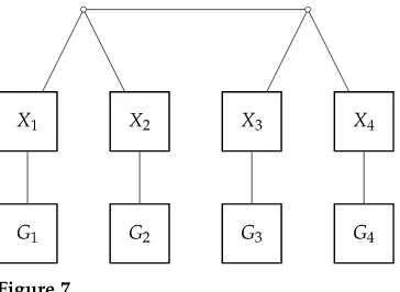
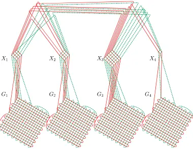
Figure 7

A tree layoutTMof cyclic permutation multigraphM(shown later in Figure 11) derived from the

tree layoutTof Figure 5.

for each edge (i,j) of G, there are interconnection edges connecting components Xi

andXj.

Interconnection edges serve two main purposes. First, they are used to connect the red and green paths withinM, so thatMsatisfies the definition of cyclic permutation multigraph. Second, the connections between component pairsXi and Xj mimic the

structure of the source graphG, as will be explained in more detail later. This second condition guarantees that an optimal tree layoutTM of M can be obtained from an

optimal tree layoutTofG, by placing eachXi andGicomponent under the leaf node

of T that is associated with vertex i of G. A simple example of the construction is schematically depicted in Figure 7.

4.2 Construction

In this section, we define precisely the grid-like graphsXiandGi, for each vertexiof the

source graphG, and outline the overall structure of the cyclic permutation multigraph Mconstructed fromG.

4.2.1 Depth-First Traversal.To be used later in our construction, we need to define a special ordering of the edges of G. We do this here by constructing a path through Gthat starts at an arbitrary vertex and visits each edge exactly twice. We adapt the standard procedure for depth-first traversal of an undirected graph. More precisely, whenever we reach a vertexi, we continue our path by arbitrarily choosing an edge

Algorithm 1Procedure for depth-first traversal ofGstarting ati

1: procedureDFS(i)

2: appendito path

3: ifeach edge (i,j) has already been visitedthen

4: return

5: foreach edge (i,j) not already visited (in arbitrary order)do

6: DFS(j)

7: appendito path

Figure 8

The path constructed by Algorithm 1 starting at vertex 1 of the displayed graph is

h1, 2, 5, 2, 1, 3, 6, 3, 7, 4, 1, 4, 7, 3, 1i.

(i,j) that has not already been visited, and move toj. If all of the edges atihave already been visited, we backtrack to previous vertices of our path, until we reach edges that have not already been visited. The path construction stops when we reach the starting vertex and all of the edges of Ghave been visited. Algorithm 1 provides a recursive procedure for the incremental construction of the path, assuming that the path is a global variable initialized as the empty sequence of vertices. A simple example is also shown in Figure 8.

Letmbe the number of edges ofG. It is not difficult to show that the path produced by Algorithm 1 is a sequence hi1,. . .,i2m+1i of vertices fromG satisfying both of the following properties.

r

ik+1=j, and there is a uniqueh∈[2m] such thatih =jandih+1=i.

r

degree of vertexjinG.)

The first bullet says that each edge ofGis traversed exactly twice, the first time in one direction and the second time in the opposite direction. The second bullet is a direct consequence of the first bullet. These properties will be used in the specification of cyclic permutation multigraphM.

4.2.2 Component Xi.The graph component Xi, i∈[n], embeds a square grid with 2di

rows and 2di columns. In addition to the edges of the grid, Xi also contains a set

of interconnection edges that connect Xi to component Gi (specified later) and that

connect Xi to all componentsXj such that (i,j) is an edge ofG. This is schematically

depicted in Figure 9. (A complete example for componentsXiandGiwill be presented

later.)

More precisely, letx(mi),nbe the vertex in themth row andnth column ofXi. Similarly,

Figure 9

GridXicorresponding to vertexiofGwithdi=3. Interconnection edges from the left column

and top row reach gridsXjfor verticesjthat are neighbors ofiinG.

r

(i)

p,1). Furthermore,Xihas an interconnection edgeα₂(i_d)_i =(x(₂i_d)_i,2di,g₂(i_k)_,1).

r

β_q(i)=(x₂(i_d)

i,q,g

(i)

1,q). Furthermore,Xihas an interconnection edge

β₂(i_d)

i =(x

(i) 2di,2di,g

(i) 1,2k).

Overall, this specification provides 4diedges connectingXiandGi. As will be discussed

later, 2diof these edges belong to the red path and 2dibelong to the green path.

For the connections between gadgetXi and other gadgetsXj, our strategy is more

involved, because we need to reproduce the topology ofGand, at the same time, we need to construct a red and a green path withinM. For each vertexjthat is a neighbor of vertex i in G, we add two red edges between the left column of Xi and the left

column of Xj, and two green edges between the top row of Xi and the top row of

Xj; see again Figure 9. Crucial to our construction, the order in which we visit the

neighbors ofiis induced from the depth-first traversal ofGspecified by Algorithm 1 in Section 4.2.1.

counts the number of interconnection edges already established for the left column (equivalently, for the top row) ofXi, at stepkof the depth-first traversal, that is, right

before the kth edge (ik,ik+1) of γ is processed. In this way, dfγ(i,k)+1 is the next

available position in the left column (equivalently, top row) ofXiwhen visiting thekth

edge ofγ.

For technical reasons, gridX1needs a special treatment: the last edge (i2m,i2m+1) inγ is used to enter gridX1for the first time, and is therefore placed at vertexx1,1(1). Therefore, all other edges ofγthat are placed atX1need to be shifted by one position. This means that we have to increase our countdfγ(i,k) by one unit wheni=1 andk<2m, and we

have to treat the case ofi=1 andk=2min a special way. Formally, fori∈[n] andk∈[2m], we define

dfγ(i,k)= 





|{k0:k0<k, i∈ {ik0,i_k0₊₁}}|, ifi>1

|{k0:k0<k, i∈ {ik0,i_k0₊₁}}|+1, ifi=1,k<2m

1, ifi=1;k=2m

We are now ready to specify the interconnection edges for Xi. Recall from

Sec-tion 4.2.1 that, for an edge (i,j) ofG, there exists a uniqueksuch thatik=iandik+1=j inγ, and there exists a uniquek0such thatik0 =jandi_k0₊₁=i.

r

γ(i,k)+1,1,x

(j)

dfγ(j,k)+1,1). Symmetrically,Xihas an interconnection edge

(x(_1,i)_df

γ(i,k)+1,x

(j)

1,dfγ(j,k)+1).

r

ihas an interconnection edge

(x(_dfi)

γ(i,k0)+1,1,x

(j)

dfγ(j,k0)+1,1). Symmetrically,Xihas an interconnection edge

(x(_1,i)_df

γ(i,k0)+1,x

(j)

1,dfγ(j,k0)+1).

Informally, this specification means that for each edge (i,j) ofG we have four inter-connection edges between Xi and Xj: two edges from when the depth-first

traver-sal first explores the edge from i to j, and two edges from when the depth-first traversal travels back from j to i. This amounts to 4di interconnection edges for

gridXi.

4.2.3 Component Gi.We now turn to (multi)graphGi,i∈[n], which embeds a square grid

with 4krows and 4kcolumns; herekis the positive integer in the input instance of the carving width problem in our reduction; see Section 4.1. We have already introduced interconnection edges α(_pi) andβ_q(i) forGi in Section 4.2.2. In addition to these edges,

we need to double some occurrences of the edges internal to the grid Gi, in order to

connect the red and green paths withinM. We remind the reader thatMis defined as a multigraph; therefore we can introduce multiple edges joining the same pair of vertices ofGi. As will be discussed in detail later, our construction always assigns different colors

(red or green) to two edges joining the same pair of vertices. An overall picture ofGiis

schematically presented in Figure 10 fordi=3 andk=5.

We first provide the specification of the red edges ofGi.

Figure 10

Grid gadgetGicorresponding to vertexi. We assumedi=3 andk=5. The red path is drawn

using a heavy red line; the green path is drawn using a dashed, heavy green line. The red path visitsGione row at a time. The only exception is at row 2k: after reaching the middle of that

row, the red path switches to row (2k+1). The path comes back to row 2konly after having completed the lower half ofGi. The green path follows a symmetrical pattern in visitingGione

column at a time, with a switch in the middle of column 2k.

r

r

r

2k+1,1,g (i) 4k,1).

This set of edges form the red extra edges ofGi. Symmetrically, for each red extra edge

Example 6

We now provide an example that uses the specifications in this and the previous section. Consider the graphGin Figure 5, and letk=4. Assume the depth-first traversal ofG that produces the vertex pathγ=h1, 2, 3, 4, 3, 1, 3, 2, 1i. FromG,k, andγwe construct the cyclic permutation multigraphMshown in Figure 11.

Let us focus on vertex 3 in G, and the associated components X3 and G3 in M. Becaused3 =3,X3has size 6×6. Because vertex 3 is connected to vertices 1, 2, and 4 in G, gridX3has two red and two green interconnection edges to each of the components X1,X2, and X4. Consider now all the edges ofGimpinging on vertex 3. These edges are visited twice by γ, in the order (2, 3), (3, 4), (4, 3), (3, 1), (1, 3), (3, 2). Accordingly, when visiting the first column of X3 from top to bottom, we touch upon the red interconnection edges for grids X2,X4,X4,X1,X1, and X2. Exactly the same order is found for the green interconnection edges, when visiting the first row ofX3from left to right.

Grid G3 has size 4k×4k, that is, 16×16. This is also the size of any other grid Gi in M. We have 2d3=6 red interconnection edges connectingG3 andX3; these are theα(3)_p edges of Section 4.2.2, forp∈[6]. Each edgeα(3)_p ,p∈[5], impinges on vertex g(3)_p,1, and edgeα(3)₆ impinges on vertexg(3)_8,1. A symmetrical pattern is seen for the green interconnection edgesβ(3)_q ,q∈[6], connectingG3andX3.

Figure 11

4.2.4 Cyclic Permutation Multigraph M.To summarize the previous sections, the cyclic permutation multigraphM contains componentsXi and Gi for eachi∈[n], wheren

is the number of vertices of the source graph G. Besides the edges of the grid-like componentsXiandGi,Malso contains some interconnection edges. More precisely, for

each vertexiofG,Mcontains 2dired edgesαp(i)and 2digreen edgesβ(qi)connectingXi

andGi. Furthermore, for each edge (i,j) ofG,Mcontains two red edges and two green

edges connectingXiandXj.

We still need to show thatMis a cyclic permutation multigraph, that is, all the edges mentioned above form a red Hamiltonian cycle and a green Hamiltonian cycle over the vertices ofM. We start by observing that, within each componentGi, these two cycles

are symmetric, in the sense that the green Hamiltonian cycle can be obtained from the red Hamiltonian cycle by switching the first and the second indices of each vertex in an edge. In other words, withinGithe green Hamiltonian cycle can be obtained from the

red Hamiltonian cycle by a rotation along the axis from vertexg_1,1(i) to vertexg(₄i_k)_,4k. This is also apparent from Figure 10. A similar observation holds for the componentsXi, as

apparent from Figure 9, and for the interconnection edges. For this reason, we outline in the following only the red Hamiltonian cycle ofM.

The red cycle ofMstarts and ends at vertexg(1)_1,1inG1. The cycle follows a depth-first traversal ofGspecified by Algorithm 1 in Section 4.2.1. Each time the depth-first traversal visits nodeiofG, the red cycle travels across one row ofXifrom left to right,

then passes throughGi, and then travels across the next row inXi from right to left,

before proceeding to the gadget for the next vertex ofG in the depth-first traversal. Exactly how the red cycle travels throughGidiffers for the firstdi−1 times thatGi is

visited and the final time; see Figure 10. The firstdi−1 times thatGiis visited, the red

cycle travels from left to right across one row, descends to the next row, and traverses it from the right to left. On the final trip intoGi, the cycle visits all the remaining rows as

follows. It travels left to right across row 2(di−1)+1 ofGi, then zig-zags across the next

2k−2(di−1)−1 rows in the upper half ofGi. Upon reaching vertexg(2ik),2k+1, coming from its right and proceeding to the left, the red cycle moves tog₂(i_k)_+1,2k+1using an edge internal to the grid. This choice is designed to ensure, for reasons that will become clear later, that none of the extra edges added to the grid underlyingGicrosses between the

grid’s four quadrants.

Next, the red cycle travels from vertexg₂(i_k)_+1,2k+1toward the right to reachg₂(i_k)_+1,4k, and then zig-zags across the next 2k−1 rows of the lower half ofGi. Upon reaching

vertexg(₄i_k)_,1, the red cycle jumps to vertexg₂(i_k)_+1,1using a single extra edge. It then travels toward the right to reachg(₂i_k)_+1,2k, moves to g₂(i_k)_,2k using an edge internal to the grid, and finally proceeds toward the left to reachg(₂i_k)_,1. This completes the last traversal ofGi

by the red cycle.

Fromg(₂i_k)_,1the red cycle leavesGiand entersXiat vertexx(₂i_d)_i,2di. It then travels across

the bottom row ofXito reach vertexx₂(i_d)_i,1, and then proceeds to visit the gadgetXjfor

the next vertexjofGin the depth-first traversal, as already mentioned.

4.3 NP-Completeness

from the carving width decision problem for a general graph. Throughout this section, we assume thatG,k, andMare defined as in the previous sections.

Lemma 2

Within a tree layoutTM of M, we can organize all vertices ofGi, for anyi∈[n], into

a (connected) subtree TGi of TM in such a way that there is an upper bound of 4kfor

the width of any arc internal toTGi and for the width of any arc connectingTGi to the

remaining nodes ofTM.

Proof

It has been shown by Kozawa, Otachi, and Yamazaki (2010) that the carving width of anm×mgrid withmeven ism. We adapt here their construction to show the statement of the lemma.

The subtreeTGi is built by dividing the gridGiinto four quadrants of size 2k×2k,

shown by black dotted lines in Figure 12. Consider first the upper left quadrant. We build a linear subtreeTULby adding vertices of this quadrant one at a time in column

major order. More specifically, we add columns of the quadrant from left to right, and we add vertices within each column from top to bottom, as shown Figure 12. We use symmetrical constructions for the bottom left quadrant, the bottom right quadrant,

Figure 12

Subtree layout for gridGi, assumingdi=k=3. The subtree layout is drawn using a thick black

and the upper right quadrant of Gi, resulting in the linear trees TBL, TBR, and TUR,

respectively. The top-most nodes of the linear treesTULandTBLare connected to a new

nodenL; similarly, the top-most nodes ofTURandTBRare connected to a new nodenR,

andnLandnRare connected together. This completes the specification of the tree layout

TGi. Finally, an extra edge is used to connect the bottom-most internal node ofTULto the

remaining nodes of the tree layoutTM. See again Figure 12.

We now prove an upper bound of 4kfor the width of any arc internal toTULand for

the width of any arc connectingTULto the remaining nodes ofTM. The binary treeTUL

has 4k2 _{leaf nodes and 4k}2 _{internal nodes. Let us name the internal nodes ofT}

ULfrom

bottom to top, using integers in [4k2_{] in increasing order. Because the width ofT}

ULdoes

not decrease at the increase ofdi, in what follows we consider the worst case ofdi=k.

Observe that the arc connecting internal node 1 to the remaining nodes ofTMroutes

4kedges ofGi, namely, the interconnection edges ofGithat lead toXi. When we move

to arc (1, 2) ofTUL, we lose the two interconnection edges impinging on vertexg(1,1i) ofGi,

but those edges are replaced by two new internal edges ofGi, namely, edges (g_1,1(i),g_2,1(i))

and (g(_1,1i),g_1,2(i)). Therefore, arc (1, 2) ofTUL still routes 4kedges ofGi. Climbing up tree

TUL at arcs (2, 3), (3, 4), and so on, shows exactly the same pattern, with two edges

impinging on the newly added vertex ofGireplaced by two new edges ofGiimpinging

on the same vertex. This process goes on until we reach the arc that connects node 4k2 (the top-most node ofTUL) to nodenL. This arc routes the 4kedges of the upper left

quadrant that reach the upper right quadrant and the lower left quadrant.

To conclude our proof, we observe that the upper left quadrant embeds any of the three remaining quadrants ofGi. Because the treesTBL,TBR, andTURare

sym-metrical toTUL, the former trees must also have an upper bound of 4k on the width

of their internal arcs as well as on the width of the arcs connecting these trees to the remaining nodes ofTM. Finally, we observe that the arc connecting nodesnLandnRalso

routes 4kedges of Gi, namely the edges from the two left quadrants to the two right

quadrants.

In the case ofdi=k, the grid componentXi is the same as the top left quadrant of

Gi. Therefore, the analysis provided in the proof of Lemma 2 can also be used to prove

the next lemma.

Lemma 3

Within a tree layoutTM ofM, we can organize all vertices ofXi, for anyi∈[n], into a

subtreeTXi ofTMin such a way that there is an upper bound of 4kfor the width of any

arc internal toTXi and for the width of any arc connectingTXi to the remaining nodes

ofTM.

The tree layout for Xi is a long chain, isomorphic to the tree layout of the upper

left quadrant ofGi in Figure 12. In what follows, we refer to the node of the layout

immediately abovex_1,1(i) as top-most, and the node immediately abovex₂(i_d)

i,2dias

bottom-most. We can now prove the correctness of our reduction for one direction.

Lemma 4

If Ghas a tree layout T of carving width k, thenM has a tree layout TM of carving

width 4k.

Proof

tree layout for each gridXiandGiunder the node ofTassociated with vertexi. As an

example, for the cyclic permutation multigraphMof Figure 11, this will provide the tree layout schematically depicted in Figure 7.

For eachi∈[n], we use the tree layoutT(Gi) from Lemma 2 and connect it to the

tree layoutT(Xi) from Lemma 3. The connection arc is created from the bottom-most

internal node of subtree TUL ofT(Gi), to the top-most node ofT(Xi). The tree layout

T(Xi) is in turn connected to the tree layoutTforG. The connection is established by

merging the bottom-most internal node ofT(Xi) and the leaf node ofTassociated with

vertexiofG.

From Lemma 2 and Lemma 3, we have that any of the treesT(Gi) andT(Xi) have

width at most 4k. The edges ofMthat are routed through the arc connectingT(Gi) to

T(Xi) are exactly the 4di≤4kinterconnection edges betweenGi andXi. The edges of

Mrouted through the connection betweenT(Xi) andTare the 4di≤4kinterconnection

edges betweenXi and all theXj forja neighbor of vertexiinG. Finally, the top-level

subtreeTwithinTMalso has carving width at most 4k. To see this, observe that for each

edge (i,j) routed by an arcaof the tree layoutTofG, the same arcain (the copy of)T used as a subtree of the tree layoutTMroutes two red and two green edges connecting

componentsXiandXjofM. Because the carving width of the tree layoutTofGisk, we

conclude that the carving width of the tree layoutTwithinTMis 4k.

We now deal with the other direction in the correctness of our reduction. We must show that ifMhas a tree layout of carving width 4k, thenGhas a tree layout of carving widthk. This will be Lemma 8, for which we will need to develop a few intermediate lemmas. We introduce our first intermediate lemma by means of a simple example.

Example 7

Consider the tree layout of grid Gi,i∈[n], that has been depicted in Figure 12 as a

subtree of a tree layoutTMofM. Letabe the arc that connects the bottom right quadrant

of the grid to the remainder of the layout. Using the notation in the proof of Lemma 2, arcacan be written as (nR,nBR), withnBRthe top-most node of linear treeTBR. Observe

that there are 4kedges ofMrouted through arca(in Figure 12 we havek=3). These are the 2kred edges that connect the bottom right quadrant with the bottom left quadrant ofGi, and the 2kgreen edges that connect the bottom right quadrant with the top right

quadrant. These 4kedges ofMare all internal to grid Gi, meaning that they connect

vertices withinGi. Finally, observe the subtree rooted at nodenBRcontains 4k2vertices

fromGi.

The special properties of arcathat we have mentioned here are not dependent on the choice of the tree layoutTM. In fact the next lemma shows that, for every choice of

a tree layout ofMhaving carving width 4k, and for every gridGi inM,i∈[n], there

always exists an arc that satisfies the properties of Example 7. Intuitively, this happens because the vertices in a grid have a relatively high degree of interconnections, and when we pick up a sufficiently large set of vertices of a gridGi, we have a large number

of edges connecting the vertices in our set to the remaining vertices ofGi. This in turn

means that, in any tree layoutTM, any subtreeTi containing a sufficiently large set of

vertices ofGimust route a large number of edges fromGithrough the arcathat connects

Ti to the rest ofTM. IfTM has bounded carving width, the edges routed through arca

saturate the width of this arc, making it impossible for other vertices not fromGito be

placed withinTi. In other words, there is always some core set of vertices fromGithat

Lemma 5

LetTMbe a tree layout ofMhaving carving width 4k. For each vertexiofG, there exists

an arcaiofTMsatisfying all of the following properties:

(i) The width ofaiis 4k.

(ii) The edges ofMrouted throughaiare all internal to gridGi.

(iii) One of the two subtrees obtained by removingaifromTMcontains only

vertices internal toGi; we call this the subtree belowai.

(iv) The subtree belowaicontains at least 4k2vertices fromGi.

Proof

For a subtreeTofTM, letLi(T) be the number of vertices ofGithat are at the leaves of

T. Consider an arcaofTM, and letT1 andT2 be the two subtrees ofTM obtained by

removingafromTM; this is exemplified in Figure 13. We say thataisbalancedforGi

if the choice ofaminimizes|Li(T1)−Li(T2)|.

The following argument is a standard one, see for instance Kozawa, Otachi, and Yamazaki (2010, Lemma 3.1). Assume thatais a balanced arc in TM. Let |Gi|=(4k)2

be the number of vertices ofGi. Without loss of generality, we assume thatLi(T1)≥ Li(T2). Because|Gi|=Li(T1)+Li(T2), this impliesLi(T2)≤ 21|Gi|. Because|Gi| ≥16, we

must haveLi(T1)>1, otherwise awould not be balanced. Then the root of T1 must have two children, rooting subtreesT₁0andT₁00ofT1; see again Figure 13. We must have Li(T10)≤Li(T2) and Li(T100)≤Li(T2), otherwisea would not be balanced. This in turn impliesLi(T2)≥13|Gi|. To summarize these inequalities, we have

1

3|Gi| ≤Li(T2)≤ 12|Gi| (6)

For each vertexiofG, we now chooseaiin the statement of the lemma to be a balanced

arc forGi. In the following discussion we focus on an arbitrary choice ofi∈[n], and

again we letT1andT2be the two subtrees ofTMobtained by removingaifromTM, with

Li(T1)≥Li(T2), so that we can use Equation (6).

a

T1 T2

T0

1

T00

1

Figure 13

Definition of balanced arcaofTMfor some gridGi. TreesT1andT2are the two subtrees ofTM

Let Sbe a grid of size 4k×4k, that is, a square grid with |Gi|nodes. It is known

that, for any choice ofsnodes fromSwith 1

3|Gi| ≤s≤ 12|Gi|, there are at least 4kedges

of Sconnecting the chosen nodes to nodes in the complement set. For this claim, see for instance Ahlswede and Bezrukov (1995) or Rolim, S ´ykora, and Vrt’o (1995). This claim must also be true for the edges internal toGi, sinceGiembeds the gridS. From

Equation (6) we then have that at least 4kedges internal to Gi are routed throughai.

Furthermore, sinceTMhas carving width 4k, the width ofaicannot exceed 4k. We then

conclude that conditions (i) and (ii) are both satisfied.

LetNibe the set of vertices ofMthat are not vertices ofGi. It is easy to see from the

specification in Section 4.2 that the sub-multigraph of Minduced byNi is connected.

(This is the very reason why we introduced the componentsXi in our construction of

M.) This implies that for any pair of vertices inNi, there exists a path inMconnecting

the two vertices that is entirely composed of edges that are not internal toGi. If both

T1 andT2have some vertex fromNi, there would be an edge not internal toGirouted

throughai, in contrast to condition (ii). We therefore conclude that one amongT1andT2 contains only vertices internal toGi, satisfying condition (iii). This subtree is called the

subtree belowai.

From Equation (6) and by our choice of T1, we have 13|Gi| ≤Li(T2)≤Li(T1). Fur-thermore, 4k2 _<1

3|Gi|, and hence both T1 and T2 have at least 4k2 vertices from Gi.

Regardless of which ofT1orT2is belowai, we conclude that condition (iv) is satisfied.

Consider a square gridQof size 4k×4k, and letdbe some fixed integer withd∈[k]. Assume that 2dvertices in the left-most column ofQand 2dvertices in the top-most row ofQhave been selected asconnector vertices. Observe that the number of connector vertices in Q is either 4d−1 or 4d, depending on whether the vertex at the top-left corner ofQis selected twice or not. LetSbe any subset of the vertices ofQ. Recall from Section 3 that theedge boundaryofSinQ, written∂_Q(S), is the set of edges ofQthat connect vertices inSand vertices inS, the complement set ofS.

Lemma 6

LetQbe a square grid of size 4k×4kand letd∈[k]. Assume 2dconnector vertices in the left-most column and 2dconnector vertices in the top-most row ofQ. Let alsoSbe a set of vertices ofQsuch that|S| ≥4k2 andSdoes not contain any connector vertex. Then

|∂_Q(S)| ≥4d.

Proof

We distinguish three cases in the following, depending on whether the setScontains any entire column and/or any entire row ofQ.

Case 1: S contains at least one entire column of Q and at least one entire row of Q. (This part of the proof is adapted from Kozawa, Otachi, and Yamazaki [2010, Propositions 4.4, 4.5, and 4.7].) Letrbe the number of rows ofQthat have at least one vertex inS. Within each such row there must be a vertex not inS, since at least one entire column ofQis not inS. This means that at least one edge of this row is in the set∂_Q(S), for a total ofredges in∂_Q(S). A similar argument applies to the number of columnscof Qthat have at least one vertex inS.

Because rows and columns have disjoint sets of edges, we have|∂_Q(S)| ≥r+c. It is well known that the arithmetic mean (r+c)/2 is always larger than or equal to the geometric mean√rc. Becauserc≥ |S|, we can write|∂_Q(S)| ≥2√rc≥2p|S| ≥2

√

Case2:Scontains at least one entire column ofQbut no entire row, or elseScontains at least one entire row ofQbut no entire column. In the first case we haver=4kand, as explained in Case 1, 4k≥4dedges in the set∂_Q(S). Symmetrically, in the second case we havec=4kand thus 4k≥4dedges in∂_Q(S).

Case3:Sdoes not contain any entire column ofQ, nor any entire row ofQ. In this case each row ofQhas at least one vertex inS. Because the connector vertices are all contained in the setS, each of the 2drows ofQthat have a connector vertex contributes at least one edge to the set∂_Q(S). A symmetrical argument applies to the 2dcolumns ofQthat have a connector vertex. Again, because the rows and the columns ofQhave disjoint edges, we conclude that|∂_Q(S)| ≥4d.

LetTM be any tree layout ofMwith carving width 4k. In Lemma 5 we associated

each vertexiofGwith an arcaiofTM having some specific properties. Similarly, our

next lemma associates each edge (i,j) ofGwith a set of four paths inTM. These paths

are routed throughaiand throughaj, and do not share any of their edges. Using this

property, we will later be able (in Lemma 8) to derive the carving width ofGfrom the carving width ofM. We use a simple example here to illustrate the special paths we are looking for.

Example 8

Consider once more the grid Gi and its subtree layout depicted in Figure 12, where

we havedi=k=3. We reportGiin Figures 14 and 15, where for convenience we have

ignored the associated tree layout. As in Example (7), consider the arc in the linear layout that connects the bottom right quadrant ofGi to the remainder of the layout.

Here we denote this arc asai. There aredi=3 neighbors of i in G, and we need to

associate four paths with each neighbor, for a total of 12 paths routed throughai. In

Figure 14

Paths starting with the red edges routed through arcaiofTM. These paths and the paths in

Figure 15

Paths starting with the green edges routed through arcaiofTM. These paths and the paths in

Figure 14 do not share any of their edges.

what follows we focus our attention on the first segment of each of these 12 paths, more precisely, the segment of these paths that starts at an edge ofMrouted throughai

and ends at some edge ofMthat leavesGito reach gridXi.

In Figure 14 we outline the first segment of six paths ofMrouted through arcai,

starting with the red edges that connect the bottom right quadrant with the bottom left quadrant ofGi. These paths reach the six vertices in the left-most column ofGithat are

connected with the gridXiand will eventually reach the gridsXjandGj, for each vertex

jthat is a neighbor ofiinG. Similarly, in Figure 15 we outline six more paths ofMrouted through arcai, starting with the green edges that connect the bottom right quadrant with

the top right quadrant ofGi. These paths reach the six vertices in the top-most row ofGi

that will eventually reach the gridsXjandGjfor each neighborjofi.

Finally, observe that these 12 paths routed throughaishare some of their vertices in

the top left quadrant ofGibut do not share any of their edges. To see this, consider the

diagonal of the top left quadrant from the bottom left corner to the upper right corner. Notice then that the paths in Figure 14 use the vertical edges ofGibelow the diagonal,

and the paths in Figure 15 use the horizontal edges below the diagonal. Similarly, the paths in Figure 14 use the horizontal edges above the diagonal, and the paths in Figure 15 use the vertical edges above the diagonal.

The next lemma generalizes the previous example, showing that for any tree layout TM we can associate each edge (i,j) of Gwith a set of four paths in Mthat are edge

disjoint. We need to introduce some auxiliary notation. LetTMandai,i∈[n], be defined

as in Lemma 5. Consider an arc (i,j) in the source graphG. A path in Mis called an (i,j)-pathforTMif it starts at a vertex inside the subtree belowai(see Lemma 5(iii) for

the definition of this subtree) and it ends at a vertex inside the subtree belowaj. We also

Lemma 7

LetTMbe a tree layout ofMhaving carving width 4k. There exists a setP of paths inM

satisfying both of the following properties:

(i) For every edge (i,j) in the source graphG,P contains four (i,j)-paths for TM.

(ii) Every two paths inP are edge-disjoint.

Proof

We call connector edges the edges of M that are not internal to any component Gi,

i∈[n]. We callconnector verticesthose vertices ofGi,i∈[n], that have an impinging

connector edge. In this way, eachGihas 4di−1 connector vertices. These are placed in

the left-most column ofGiand in the top-most row ofGi. We claim that, for eachi∈[n],

the connector vertices ofGimust all be outside of the subtree ofTMbelowai. To see this,

let us assume that some connector vertex ofGiis found inside the tree belowai. Because

connector vertices are connected to vertices outside ofGi, there would be a vertex not

internal toGi inside the tree belowai, against Lemma 5(iii), or else there would be a

connector edge routed throughai, against Lemma 5(ii). We therefore conclude that the

connector vertices ofGimust all be outside of the tree belowai.

The idea underlying the proof is to define each (i,j)-path inP as the concatenation of three sub-paths, calledsegments, specified as follows.

r

and this is also the starting vertex of the segment. Furthermore, the segment only uses edges that are internal toGi, and ends with a connector

vertex ofGi.

r

r

subtree belowajis the end vertex of the segment.

From now on, we focus on a specific vertexiofGand prove the existence of 4di edge

disjoint (i,j)-paths for verticesjthat are neighbors ofiinG. We do this by separately specifying the three segments of the paths.

First segment. From Lemma 5(ii), there are 4kedges internal to Gi that are routed

through arcai. We know that k≥di, since the carving width of a graph is always at

least its degree. Thus we start our segments with any choice of 4didisjoint edges routed

through arcai. We now show that these edges can be extended to 4disegments that reach

the 4di−1 connector vertices ofGi, without sharing any of their edges. We do this by

reducing our problem to a network flow problem.

If we assume that edges ofGihave flow capacity of one, each segment corresponds

to a flow throughGi having capacity one. The existence of 4di edge disjoint segments

is then equivalent to the existence of a flow of capacity 4difrom the subtree belowaito

the 4di−1 connector vertices ofGi. LetV(Gi) be the set of vertices ofGi. The max-flow

source vertices on one side and the target vertices on the other side has capacity not less than 4di.

In our specific case, consider the square gridQunderlying componentGi. LetS⊆

V(Gi) be a vertex set including all the vertices in the subtree belowaiand excluding all

the 4di−1 connector vertices ofGi. If we can show the relation

|∂_Q(S)| ≥4di (7)

for any choice ofSas before, then we have proved the existence of the desired 4diedge

disjoint segments.

In order to prove Equation (7), we observe that the set of vertices in the subtree below ai has size greater than or equal to 4k2, by Lemma 5(iv). Furthermore, observe

that there are 2di connector vertices of Gi in the left-most column of Qas well as 2di

connector vertices in the top-most row. Under these conditions, we can apply Lemma 6 to the gridQ, withd=di≤k, and derive Equation (7). We then conclude that there exist

4diedge disjoint first segments starting at vertices in the subtree belowai, as desired.

Second segment. As already observed in Section 4.2.2, for every connector vertex in the left-most column ofGi there is a red segment to some connector vertex in the

left-most column ofGj, wherejis some neighbor ofiinG. Symmetrically, for every connector

vertex in the top-most row ofGithere is a green segment to some connector vertex in

the top-most row of someGj. This provides a total of 4disegments. These segments are

all edge disjoint, by construction of the componentsXh,h∈[n], and by construction of

the interconnection edges.

Third segment. We observe that the third segment of an (i,j)-path is the reversal of the first segment of a (j,i)-path. Therefore we can use our argument for the first segments to show the existence of 4diedge disjoint third segments ending at a vertex in the subtree

belowaj.

To summarize, for each i∈[n] we have shown the existence of 4di edge disjoint

(i,j)-paths for verticesjthat are neighbors ofiinG, to be added to setP. To complete the proof, we observe that two paths inP having disjoint start vertices must have edge disjoint first segments, since these segments are defined for edges that are internal to different components Gi. A similar argument applies to the third segments of paths

having disjoint end vertices.

Lemma 8

IfMhas a tree layoutTM of width at most 4k, thenGhas a tree layoutTof width at

mostk.

Proof

For eachi∈[n], let arcaiand the subtree belowaibe defined as in Lemma 5. We denote

byr(ai) the root of the subtree belowai. The tree layoutTofGis constructed fromTM

as follows.

r

fromTMall the arcs of this subtree and all of its nodes butr(ai).

r

nodesr(ai) andr(aj). We remove fromTMall nodes that are not in any such