The Perils of Modelling How Migration
Responds to Climate Change
Feng, Bo and Partridge, Mark and Rembert, Mark
The Ohio State University
1 November 2016
Online at
https://mpra.ub.uni-muenchen.de/77059/
The Perils of Modelling How Migration Responds to Climate Change
by
Bo Feng, Mark Partridge, Mark Rembert
Abstract
The impact of climate change has drawn growing interests from both researchers and
policymakers. Yet, relatively little is known with respect to its influence on interregional
migration. The surge of extreme weather conditions could lead to the increase of forced
migration from coastal to inland regions, which normally follows different patterns than
voluntary migration. However, recent migration models tend to predict unrealistic migration
trends under climate change in that migration would flow towards the areas most adversely
affected. Given the great uncertainty about the magnitude and distribution of severe weather
events, it is almost impossible to foresee migration directions by simply extrapolating from
the data on how people have responded in the past to climate and weather. For example,
weather events will likely be far outside of what has been observed. Other issues include a
poor climate measures and a poor understanding of how climate affects migration in an
entirely different structural environment. Unintended consequence of public policies also
contributes to the complication of predicting future migration pattern. In this paper, we
survey the limitations of existing climate change literature, explore insights of regional
I. Introduction
We live in an age of accelerating climate change. According to the National Climate
Assessment report, the average U.S. temperature has increased by 1.3。F to 1.9。F since
1895.1 Global warming has accelerated in the most recent decade, with the highest average
global temperature ever recorded being in 2015. Extreme weather conditions including
intense heat waves, flooding, hurricanes and severe storms, are expected to increase in
frequency due to climate change, affecting people living in both coastal and inland areas
(Melillo et al., 2014). Because firm and household migration is a key adaptive response to
climate change, we need accurate predictions of migration to assess the future costs of
climate change in order to craft effective policy. Though our emphasis is on the United
States, the points we make about modeling and research needs apply to all affected countries.
First, issues arise when studies on the cost of climate change fail to accurately
incorporate the adaptive mechanisms into their model for how households and businesses are
likely to behave, most notably by migration to less affected regions. When facing climate
change, people can choose either to stay in the most affected areas and pay a higher price to
mitigate such change through certain adaptive technology, or to migrate to other locations less
negatively impacted by climate change. The ultimate decision depends on the relative costs of
adaptive technology versus migration costs.2 People would choose to stay instead of migrating
if adaptation is less costly (Reuveny, 2007). Just as the spread of air conditioning and improved
public health efforts—such as controlling malaria—has contributed to the population growth
in the American South (Rappaport, 2007; Sledge and Mohler, 2013), new technologies could
lower future adaptation costs and enhance human ability to cope with extreme climate events.
When an analysis does attempt to incorporate migration into climate change models, it
often relies upon assumptions that can produce misleading results. For example, it is often
1 Melillo, Jerry M., Terese (T.C.) Richmond, and Gary W. Yohe, Eds., 2014: Climate Change Impacts in the United States: The Third National Climate Assessment. U.S. Global Change Research Program, 841 pp. doi:10.7930/J0Z31WJ2.
http://nca2014.globalchange.gov/report
assumed that migration will continue based on past trends regardless of how climate change
alters the attractiveness of destinations and origins. Technological development, government
policy, and improving relative climate conditions in other parts of the country are all factors
that could impact how climate change affects migration and the costs incurred by households
and businesses; yet these factors are absent in our current migration models. Likewise, an
understanding of how to measure climatic attractiveness to business and households is typically
based on prior climate behavior; yet climate change will produce negative events outside of the
range of previous experience, making it hard to model without knowing how people respond.
Current migration models are unable to incorporate the more extreme possibility of massive
forced climate migration away from areas that are severely impacted.
In general, we have a good understanding of the response of migration to natural
amenities for the latter 20th century and early 21st century. However, while it is tempting to
simply apply what we have observed from the second half of the 20th century and the first part
of the 21st century to make our climate-change migration predictions, we should do so with
caution. Indeed, as we will discuss, if we had asked economists in 1940 to predict U.S. regional
population dynamics up through 2016, they would have been very wrong. Why do we think
that economists of today would do much better in making long-run forecasts of events that are
so much more challenging due to the distinctive features of climate change as well as the
normal “unknowable” features of future economic and technological events? Even with new
insights into the drivers of U.S. migration patterns in recent decades, unforeseen innovations
that will affect migration are difficult to anticipate and incorporate into our models. Indeed, the
climatic changes on the horizon are so structural, that previous reduced form findings unlikely
apply.
Researchers and policymakers are left with analysis that is incomplete and inaccurate.
Yet, there is no easy solution to the dilemma. For example, imagine regional economists of the
early 1940s trying to understand regional growth and migration 75 years in advance.
differential regional performance was relative incomes and job growth—i.e., a narrow
firm-side perspective. However, technological innovations like air conditioning and advancements
in public health along with rising incomes that allow households to “consume” more natural
amenities (a normal good) have resulted in U.S. regional economic growth that has been
dominated by natural amenity migration to nice climates, mountains, nice landscapes, lakes,
and oceans (Partridge, 2010). Partridge (2010) notes that models that stress job creation or
agglomeration such as the New Economic Geography would have predicted exactly the
opposite of what actually happened. Fortunately, there is the spatial equilibrium model which
has served economists well in understanding U.S. migration.
Even with better theoretical models, the large structural changes in climate, technology,
and possibly even in governance means that we still do not know the parameters to put into the
underlying structural equations that may form an analytic model. While forecasting future
migration is a “wicked problem,” we will highlight the need to incorporate adaptive behavior
like migration into our climate change models, and then discuss where some of our blind spots
might lie so that we can make more accurate future predictions.
In section II, we first discuss the spatial equilibrium model as a guide to understanding
regional economic patterns in advanced countries. Then we will highlight a related household
decision-making model proposed by Kahn (2014) as a way to model decisions under climate
change. Section III will discuss how past and current trends fit into the spatial equilibrium
model and then describe why these past regional trends do not help us understand how future
migration will respond to future climate change. We then assess how recent climate change
research allows us to understand the linkage between migration and climate change. Section
IV then describes some other migration and policy issues that will further affect how future
regional forecasts are modelled. The final section discusses priorities for future research.
II. Theoretical Framework: Spatial Equilibrium Model.
workhorse theoretical framework in understanding regional (subnational) migration patterns.
The impetus for a new theoretical framework that became the SEM occurred as economists
theoretical a priori prediction that relative employment and productivity growth (solely)
drove regional migration patterns was contradicted by the early Post War movements to the
Sunbelt and Mountain West (e.g., Graves, 1976, 1979). One big theoretical addition is that
households maximize utility and not just some simple function of income. While income is
one component of utility, there clearly are other quality of life factors that affect household
utility.
Spatial equilibrium is a condition that neither households nor firms have the incentive to
relocate to another location. Simply, households’ utilities are equalized across space in
equilibrium. The simplest structural SEM can be explained by the equilibrium of labor
demand and supply in a locality (e.g., Roback, 1988; Partridge and Rickman, 2003; 2006).
Following on the work of Graves (1976, 1979) and others, this idea was first fully formalized
by Roback (1982) followed by many subsequent improvements (e.g., Beeson and Eberts,
1989; Glaeser and Gottlieb, 2009). Of course, it is unlikely that a regional system is fully in
equilibrium at a given moment, but the SEM has proved invaluable to predicting regional
growth paths and net migration patterns in response to SEM disequilibrium.
The SEM is based off of the assumptions are that 1) workers are identical and completely
mobile;3 2) firms produce a numeraire traded composite good X, the price of which is
determined on an international market; 3) return of capital is equalized everywhere; and 4)
workers consume X and non-traded housing land (Beeson and Eberts, 1989). Then in spatial
equilibrium, the indirect utility function can be written as
𝑉𝑖(w, r; S)= 𝑉𝑁
Where i is region, w is wage rate, r is the price of housing land, and S is site-specific
amenities. 𝑉𝑁 is the representative national utility level. The equation shows that if there is perfect mobility of households and firms, then prices will adjust and households will move
3The assumptions that workers can be heterogeneous can be easily incorporated in the model at the expense of
until equilibrium is reached and utility equals the national average across all locations.
Indeed, a key feature that determines the accuracy of the SEM model for prediction and
policy is the degree that households (and firms) are perfectly mobile to arbitrage utility (and
profit) differentials.
Since the production is assumed to be constant returns to scale, the cost function (or the
profit function works as well) can be normalized to a unit cost function without loss of
generality. Thus, the unit cost function for region i can be written as
𝐶𝑖(w, r; S)= 1
in which the notation is the same as above. Likewise, because of perfect mobility of factors of
production, firms will move between regions to arbitrage differences in the cost of
[image:7.595.154.433.450.735.2]productions until the unit cost function for a region i equals one across the country.
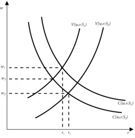
Figure 1, Determination of Equilibrium Wages and Rents
Figure 1 shows the equilibrium for two locations 1 and 2, in which the difference is that
the site specific amenity for 2 is greater than for 1 (S2>S1). By assumption VS >0 and Cs >0 or
S is a household amenity and a firm disamenity—e.g., something like clean air and costly
pollution regulations). The iso-indirect utility function is upward sloping as households are
willing to accept higher wages as a tradeoff for higher housing costs, all else equal. The
iso-cost function is downward sloping in that if land iso-costs fall, then wages will have an offsetting
increase to keep costs constant at one. In the equilibrium, wages and rents are such that the
indirect utility function crosses the unit cost function.
It is easy to see that places with natural amenities tend to have higher housing costs and
lower wages. However, migrants are not necessarily drawn to places with high nominal or
real wages, which could imply a significant compensating differential for site-specific
disamenities. Shocks to the system lead to price changes as well as migration/relocation of
factors of production to restore equilibrium (Glaeser and Gottlieb, 2009).
Kahn (2014) extends the SEM by modeling the decision of households to avoid the
negative effects of climate change by either moving or adopting measures which reduce climate
disamenities in their current location. In Khan’s model, each household i at location j at time t
chooses a combination of location, private consumption, and investments in self-protection to
maximize its utility:
𝑈(𝑖, 𝑗, 𝑡) = 𝑚𝑎𝑥 𝑝(𝑟𝑖𝑠𝑘𝑖𝑗𝑡,𝑒1) ∗ 𝑈(𝐶, ℎ(𝑎𝑚𝑒𝑛𝑖𝑡𝑦𝑖𝑗𝑡, 𝑒2))
𝑠. 𝑡. : 𝐶 = 𝑖𝑛𝑐𝑜𝑚𝑒𝑑𝑗𝑡− 𝑟𝑒𝑛𝑡𝑖𝑗𝑡− 𝛿𝑡∗ 𝑒1 − 𝛾𝑡∗ 𝑒2
𝑟𝑖𝑠𝑘𝑖𝑗𝑡 𝑎𝑛𝑑 𝑎𝑚𝑒𝑛𝑖𝑡𝑦𝑖𝑗𝑡 are attributes of a location. The possibility of avoiding certain location
specific life threatening risk, 𝑝(𝑟𝑖𝑠𝑘𝑖𝑗𝑡, 𝑒1) is a function of both risk and investment 𝑒1in self-protection measure 𝑒1 at price 𝛿𝑡, to reduce risk, such as insurance. ℎ(𝑎𝑚𝑒𝑛𝑖𝑡𝑦𝑖𝑗𝑡, 𝑒2) is the Becker Household Production function, which describes how household produces “comfort”
by selecting a combination of amenities. The comfort of a household can also be improved by
2014).
Based on Kahn’s model, the appropriate way to analyze the impact of climate change
is through an expenditure function approach and estimating individual willingness to pay
(WTP) to change disamenities (migration, self-protection investment 𝑒1, and technology investment 𝑒2), because climate change will inevitably shift the distribution of locational attributes, 𝑟𝑖𝑠𝑘𝑖𝑗𝑡 and 𝑎𝑚𝑒𝑛𝑖𝑡𝑦𝑖𝑗𝑡(Kahn, 2014). Kahn’s extension of the SEM model is useful in that it directly incorporates how investment, risk, and changing amenities affect location
decisions. Yet, while this extension provides an improved framework for modeling how
households might behave in response to climate change, applying the model to develop
predictions faces several challenges addressed in the next section.
III. Recent Migration Trends.
We now discuss migration patterns since the 1950s to illustrate the connection to the SEM
and to appraise whether these trends are consistent with adaptive responses to emerging climate
change. A key pattern of U.S. migration flows is long-term persistence. Places that grew fast
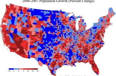
in the mid-20th century were (are) also likely growing fast in the 21st century. Figure 2 shows
that much of the population growth between 1950 – 2000 occurred in Southern Sun Belt states,
the Mountain West, and high-amenity coastal areas in the South Atlantic and Pacific coasts.
Likewise, the growth of the largest core cities such as New York, Boston, Chicago, and Detroit
greatly slowed as population redistributed west and south to new cities such as Orlando,
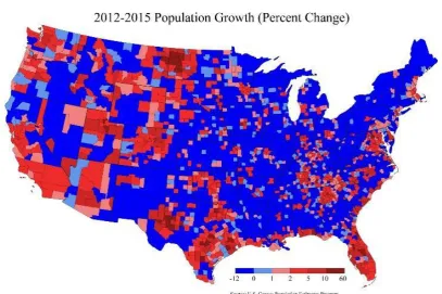
Phoenix, and Atlanta (Partridge, 2010). Figure 3 shows that this trend continued unabated into
the early 2000s up to the housing bust beginning in 2007. During the Great Recession, a pause
took place because the most affected places hit by the housing crash were typically
high-amenity areas. Yet, we show that after the housing market and economy stabilized in circa
Figure 2.
[image:10.595.115.503.488.741.2]* Source, U.S. Census Bureau.
Figure 3.
* Source, U.S. Census Bureau.
Figure 4.
[image:11.595.83.491.452.723.2]* Source, U.S. Census Bureau.
Figure 5
Figures 4 and 5 illustrate the persistence in migration. Even after the major shocks of a
housing bubble/bust and the Great Recession, long-term migration patterns reasserted
themselves after about five years. At least superficially, this may suggest that it will take a
massive shock to reverse such trends, at least until we fully reach spatial equilibrium. Figure 4
shows that the 2000-15 growth patterns mimic the 2012-15 growth patterns—which follow
closely the 2000-07 and 1950-2000 patterns. The only exceptions is that during the circa
2005-2015 period, much of the Great Plains experienced a positive commodity boom including
agriculture, oil and natural gas. Thus, those regions had much more positive growth rates than
its norm. With the recent conclusion of that commodity super-cycle, those patterns should
revert in the long term.
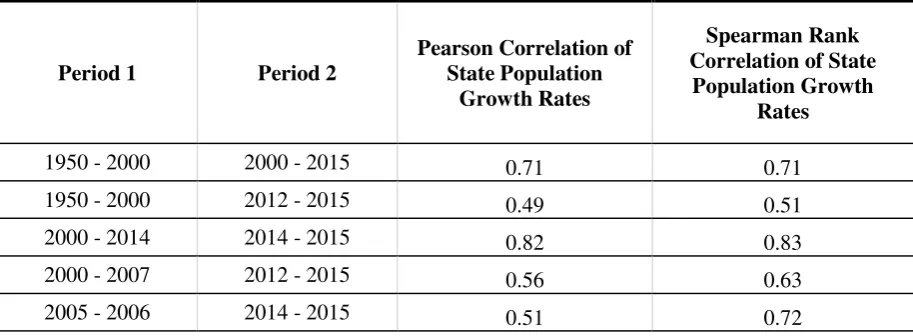
Table 1 shows that at the state level, correlations of population growth and the respective
state rank correlations over several different time periods over 1950-2015. The results illustrate
that modern U.S. regional growth patterns are very persistent even when considering growth
in the 1950-2000 period to growth in the 2012-2015 period. This strong correlation prevails
even with the super-commodity boom leading to faster than normal growth rates in the interior
of the country. These persistent patterns are consistent with the SEM, in which natural
amenities attract people to areas that are relatively “nice.” Conversely, they are inconsistent
with disequilibrium economic demand shocks driving these regional growth patterns; that
would suggest very random distributions as regions and their businesses experience shocks at
a different pace—i.e., it is not that actors aren’t responding to differential regional economic
shocks, rather if differential economic shocks were primarily at work, then the growth patterns
Table 1. The Correlation of State Population Growth Rates Over Time
Period 1 Period 2
Pearson Correlation of State Population
Growth Rates
Spearman Rank Correlation of State
Population Growth Rates
1950 - 2000 2000 - 2015 0.71 0.71
1950 - 2000 2012 - 2015 0.49 0.51
2000 - 2014 2014 - 2015 0.82 0.83
2000 - 2007 2012 - 2015 0.56 0.63
2005 - 2006 2014 - 2015 0.51 0.72
Source: US Census Bureau Population Estimates Program
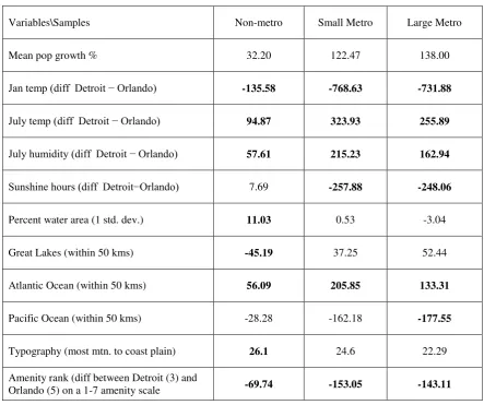
Table 2 shows the importance of amenities using the 1950-2000 population growth results
from Partridge et al. (2008). We compare outcomes of places that have the same “low-natural amenity” values such as Detroit to places with the “high-natural amenity” values of Orlando,
Florida. The table uses the amenity values for Detroit and Orlando and then applies these values
to Partridge et al.’s (2008) population change regression coefficients from nonmetropolitan,
small metropolitan (counties in metropolitan areas with less than 250,000 people in 1990) and
large metropolitan samples (counties in metropolitan areas with more than 250,000 people in
1990).
The results consistently show large statistically significant differences between places with
amenity characteristics of Detroit and Orlando. For example, the average differences in January
temperature is associated with 135% faster growth in non-metro counties that had Orlando’s
January temperatures versus Detroit’s, with corresponding gaps of about 750% for the metro
samples. However, some differences are offset by summer temperatures and humidity in places
like Orlando.4 In fact, it is apparent that urban areas are much more affected by climate effects,
which means urban growth patterns will likely see the biggest migration adjustments due to
climate change.
Table 2, Difference in Population Growth over 1950-2000
Variables\Samples Non-metro Small Metro Large Metro
Mean pop growth % 32.20 122.47 138.00
Jan temp (diff Detroit − Orlando) -135.58 -768.63 -731.88
July temp (diff Detroit − Orlando) 94.87 323.93 255.89
July humidity (diff Detroit − Orlando) 57.61 215.23 162.94
Sunshine hours (diff Detroit−Orlando) 7.69 -257.88 -248.06
Percent water area (1 std. dev.) 11.03 0.53 -3.04
Great Lakes (within 50 kms) -45.19 37.25 52.44
Atlantic Ocean (within 50 kms) 56.09 205.85 133.31
Pacific Ocean (within 50 kms) -28.28 -162.18 -177.55
Typography (most mtn. to coast plain) 26.1 24.6 22.29
Amenity rank (diff between Detroit (3) and
Orlando (5) on a 1-7 amenity scale -69.74 -153.05 -143.11
* Source: Partridge et al. (2008).
* Note: Boldface indicates significant at 10% level. The difference between Detroit and Orlando uses their actual values. “1 std dev.” represents a one-standard deviation change in the variable. The models were re-estimated with USDA ERS amenity rank replacing all 9 individual climate/amenity variables to calculate the amenity rank effects (available online at ERS). The amenity scale is 1=lowest; 7=highest.
As indicated above, strong underlying pressures cause migration to the Sun Belt, the arid
Mountain West, and to coastal regions that are likely to be the the most exposed to excessive
heat, large storms, and periods of extensive drought from future climate change. Thus, people
are moving to the exact places that will experience the highest costs of climate change, meaning
that migration patterns since 1950 are exacerbating the future costs of climate change with
of climate change will be more apparent, people will begin to reverse trends and begin (net)
migration to the Northern areas and places that will be less affected by climate change.
However, these patterns do suggest that current migration patterns are unsustainable, at least
in some dimension.
For public policy purposes, it is urgent to determine when migration trends will slow down
and reverse due to ongoing climate change as well as to find the right market signals to better
incentivize these movements—e.g., higher housing insurance premiums on the exposed South
Atlantic and Gulf coasts, higher state and local taxes to provide adaptive infrastructure and
public services, etc.
There are several factors that will make it challenging for economists and planners to
predict future migration patterns. In Section IV, we will discuss some challenges that will need
to be much better addressed if economists are going to produce migration forecasts that are
precise enough to be useful to policymakers.
IV. Challenges to Predicting Future Migration Flows.
The first challenge economists face is the difficulty of predicting future technological
changes and productivity changes that will affect real household income, in which natural
amenities being a normal good, would affect how fast and to what extent households will
respond to future climate change through migration.
The second challenge facing economists is developing new climate measures. In order to
parametrize a model like Khan’s, detailed data on climate and preferences is needed. Accurately estimating a location’s 𝑟𝑖𝑠𝑘𝑖𝑗𝑡 and 𝑎𝑚𝑒𝑛𝑖𝑡𝑦𝑖𝑗𝑡 requires detailed data, though at
the moment, we are not exactly sure what measures we need. Similarly, economists currently
rely on climate measures such as average daily-high January or July temperature, number of
precipitation days, or temperature variation—which works very well in explaining how
weather has affected utility and migration since World War II. While average July
“unpleasant” climate events associated with climate change, backward looking research
would not be very useful in developing the right measures of whether extreme heat is an
accurate measure—i.e., is it numbers of days over (say) 30C or 40C, does it include heat
indices with humidity, or is average July high temperature sufficient? We simply do not
know the right measures for excessive heat episodes that seem to be in our future and looking
backward is unlikely to provide much guidance because excessive heat has not been
anywhere near the issue that it will become.
Using the empirical results produced by current migration models, increasingly warm
weather in the Sunbelt, Gulf, and Mountain West would attract population and people would
keep swarming to places experiencing relatively rapid climate warming (and other issues),
which does not seem plausible if climate forecasts are accurate. Thus, it is urgent to discover
to what degree do negative hot-summer effects begin to overwhelm the positive effects of
warm winters in terms of net-migration. We simply do not know given that such a figure is
far outside the range of past observations.
Another seeming feature of climate change is greater variability of adverse events such
as droughts, storms, tornados, hurricanes, etc. However, droughts are associated with clear
skies and low humidity that is currently associated with positive net migration. Likewise,
given the pattern of hurricanes of the last 50 years or so, places with more hurricanes tend to
be the same places that attract people today in the Gulf and South Atlantic regions. That is,
based on current empirical modelling, areas facing the most severe effects of climate change
would still attract migrants.
Thus, we need to know two things in order to understand how climate change will
directly affect migration as an adaptation response. First, we need to develop better measures
of the climatic conditions associated with climate change. Second, with such measures, we
can better assess the tipping point where these conditions are associated with positive
migration to where they become a net negative.
incorporating external unknowns like government interventions that could have a significant
impact on the predictions that we might draw from a model such as Khan’s (2014). Given that
public policy is inherently endogenous to many of the same unknown factors including the
exact climate change effects, technological change, and other factors, it is nearly impossible to
model the effects and unintended consequences of public policies.
One particular important issue is the degree that all levels of government, but especially
the federal government, subsidizes and supports infrastructure development and rebuilding in
the most affected areas. Such policies would subsidize and maybe even reinforce population
movements that encourage more people to reside in the most adversely affected areas, which
is exactly the opposite of what is good public policy—i.e., more people and economic activity
is then exposed to adverse climate change effects, further increasing losses and government
expenditures. For example, if the federal government builds a seawall to protect Florida, that
would encourage more people to live there. Such moral hazard effects are particularly
exacerbated when the central/federal government pays for such disaster prevention or disaster
recovery efforts. If local taxpayers and households faced the costs of living in hazard prone
areas, then fewer people would move to places, reducing the adaptation and mitigation costs.
Further complicating matters is the contradictory desire of many state and local
politicians to develop their local economy and create jobs in the short term (or perceived to
have created jobs), potentially impairing the interest of the general public in the long run. That
is, rather than focusing on long-term policies that may help their local communities address
climate change and community resilience, they instead focus on efforts to boost short-term job
creation. For example, they may encourage short-term economic development and
infrastructure provision even if those plans run counter to the needs to shift activity from the
most affected areas such as along South Florida beach-front property. Overall, this means that
key parameters of government policy responses to climate change are unavailable in modelling
climate-change adaptation migration.
effectively make predictions using a model such as Khan’s (2014) because we are unable to precisely estimate a household’s migration, self-protection investment 1, and market
investment2. Most studies estimating the WTP to avoid the effects of climate change only
adopt first-stage hedonic model, in which 1 and 2 are assumed to be constant over time
(Kahn, 2009; Burke et al., 2009; Deschenes and Greenstone, 2014; Albouy et al., 2016).5 Yet,
this approach will overestimate the costs of climate change because it fails to model the fact
that household behavior will change as the “rules of the game” change—i.e., Khan’s (2014)
Lucas Critique that reduced-form parameters from a hedonic model will change as structural
conditions change. Factors like the changing climate or technological change will cause the
structural parameters to change and households will alter their investment in self-protection
and disamenity migration responses (1 and 2). Unfortunately, more data alone is likely to
solve this problem. Instead, we would need data on future technology and future preferences
(and preferably actual observations), which is impossibly unavailable at the moment. While
simulations can “plug” in some values, they are educated guesses at best if not outright
misleading in other cases.
V. Existing Research in Light of Theoretical and Methodological Concerns.
Given these concerns we raise, we now examine how these concerns relate to the
existing related climate change literature. In this, we are not necessarily questioning the
technical rigor of this research, rather we comment on the data and assumptions employed.
The existing literature paints a gloomy picture of our future under climate change in which
temperature outside a narrow range (18。C ~ 20。C) would reduce labor productivity (Heal and
Park, 2015), raise mortality rate (Deschenes and Greenstone, 2011), reduce agriculture and
industrial production (Dell et al., 2009, 2012; Park, 2015), decrease national income (Hsiang,
2010; Deryugina and Hsiang, 2014; Dell et al., 2009, 2012; Colacito et al., 2016), slow
5This model is primarily a framework to analyze the future impact of climate change, not anchoring spatial equilibrium.
economic growth (Dell et al., 2009, 2012) and even increase social instability (Burke et al.,
2009).
Dell et al. (2009) use subnational data for 12 countries in Americas and find that in 2000,
national income drops 8.5% per degree Celsius rise in temperature. Dell et al. (2012) take
advantage of year-to-year temperature fluctuation within countries and find one degree
Celsius increase in temperature on average reduce GDP growth by 1.3% in a given year.
Their results seem to confirm the long observed relationship that hot-climate countries tend to
be poor (Dell et al., 2009).
Attributing a low economic growth to the weather oversimplifies the relationship
between climate and human activities. For example, predicting the cost of climate change
should not be based on past correlations that will likely change, but a genuine causal
relationship. More importantly, such results for the U.S. are inconsistent with the SEM.
Again, there is evidence that under contemporaneous weather conditions, people trade off
lower incomes to live in nice warm weather (especially in the winter), as predicted by the
SEM. That is, people in Southern U.S. climates would have lower income than those who
live in more harsh climates (cet. par.), but in spatial equilibrium, utilities are equalized across
the country. Thus, the lower incomes in warm Southern climates are not associated with
lower welfare.
It can be extremely misleading to interpret subnational correlations between income and
climate as causal in a spatial equilibrium context because income serves as a compensating
differential. Additionally, there is likely further heterogeneity because wealthy countries are
much more likely to adapt better and/or affordable technologies (e.g. air conditioning) to
offset the negative effects of high temperatures (Kahn, 2005). Indeed, a simple example can
show why such analysis is not applicable.
Assume that in a location with a temperate climate, the average summer temperature is
25C with a relatively small variation. Of course, given the current climate, businesses would
because it is so rare. However, in a climate change regime, future businesses in this location
would adapt and be much more prepared for heat waves and any output declines would be
limited.
Deryugina and Hsiang (2014) apply a difference-in-difference approach to estimate
annual income growth of U.S. counties during 1960-2000. Finding a negative link between
average daily temperature and productivity, they claimed the results are causal, though again
the results can easily be explained in a SEM framework to warm southern weather. They also
separately estimate income-temperature relationship for each decade in fear that might be
affected by adaptation strategies, and find no significant difference from pooled estimation,
though it is unclear what adaptation strategies were being taken in the 20th Century to the
very initial signs of climate change.
Colacito et al. (2016) also examine how temperatures have historically impacted the
U.S. economy. With both time-series and panel-data approaches, they find that higher
average summer temperature reduces the growth rate of state-level output. More importantly,
they also predict a one-third reduction in U.S. economic growth would result from rising
temperatures over the next century. Again, interpreting these results in the context of spatial
equilibrium can produce a completely different interpretation about welfare. In addition,
during the past with a more climate-stable history, such relationships may appear, but again
there is a need to be cautious as consumers and producers adapt new (unknown today)
technologies. Increasing awareness of changing climate and the demand for related
technological innovations are more likely to shift household behavior and lower the cost for
future adaptation technologies to a degree that one degree temperature increase will not be as
significant as in the past, though it would be very hard to predict how that might affect
migration patterns. For instance, one extremely simple change that we expect is that rather
than the winter months being when employment and production tend to fall., it will be the
There have been several hedonic studies of the effects of climate change. For one,
Kahn (2009) estimates a first-stage hedonic model (Rosen, 1974; Roback, 1982) to find the
impact of climate change on the real estate market. The impact is calculated by multiplying a
hedonic real estate gradient with the difference between the future and current climate index,
under the assumption that household behavior is held constant. Albouy et al. (2016)
developed a quality of life index to measure WTP for nicer weather, and finds an annual
1%-4% of income loss by 2100 given no change of technology and preference. Deschenes and
Greenstone (2014) and Burke et al. (2009) adopt similar approach and estimate the climate
change effect on mortality rate and civil war occurrence separately. Deschenes and
Greenstone (2014) also predict an increase of location specific mortality rate by 3% at the
end of the century under climate change, while Burke et al. (2009)claim the climate change
will very likely cause social instability and induce more civil war in Sub-Saharan Africa. Yet
again, following Kahn (2014), such reduced-form approaches overestimate the cost of
climate change, as households will be able to foresee the change of locational attributes and
adjust their self-protection investment, and the market will be able to invest in new
technology to offset negative impact of climate change. Likewise, hedonic models are only
accurate for marginal changes, which do not describe climate change.
Fan et al. (2016) use 2-stage random utility sorting model to estimate the WTP to
avoid additional day of extreme weather. While such results potentially improve upon
first-stage hedonic estimation, there remains the other problems we mentioned about not knowing
what the future entails.
In summary, the existing literature estimating the costs of climate change are primarily
static using backward-looking parameters and measures, as well as quite often not
incorporating the implications of the SEM for an advanced economy such as the U.S. As
more people make their decisions based on climate change, more R&D into new adaptive
lower than migration costs. In such a scenario, very little migration may occur. Nonetheless,
we simply do not know what will happen.
V. Climate Change in Light of the Related Economic Shock Literatures.
The relationship between natural amenities and migration is well established, but there
are other related literatures that may help inform how climate change will affect migration. For
example, the persistence of returning to long-term economic growth paths after regions are
impacted by extreme shocks has been demonstrated in a variety of cases.
For example, during the late 1980s and 1990s, Congress established a process for
realigning military bases known as BRAC (Base Realignment and Closure). This process led
to the reduction or closure of 97 major military installations across the US, with net loss of
military and defense civilian employment of more than 4,000 employees per base, representing
significant economic shocks to local economy where the bases were located (especially in rural
communities where many of the bases were located). In a representative study in this literature,
Poppert and Herzog Jr. (2003) consider the effect of these closures on local employment. They
find that within two years, the downsized employment at the military facility produced positive
in-direct employment effects. This was particularly true when former military facilities were
repurposed for other uses that were better connected to the regional economy. One implication
is that communities can recover from large economic shocks; another is that the persistence
behind regional economic growth could hamstring the needed adjustments from most to least
affected areas.
There has been significant research on the effects on natural disasters on economic events
such as how storms and droughts will impact migration patterns. Fussell et al. (2014) explore
how the pre-storm migration systems related to the post-disaster mitigation system following
Hurricane Katrina and Rita. They find that the migration system following the storms became
more concentrated and intense. In-migration from nearby counties to disaster affected counties
increased significantly during the recovery period as displaced households returned home and
from rural areas to urban areas intensified within the disaster areas during the recovery period.
These findings challenge fears that extreme weather events like storms will permanently
displace large populations. Instead, they suggest that the effects of even large shocks like
Hurricane Katrina tend to be temporary. While such results may have implications for
regionally concentrated storm events, they are considerably less applicable to widespread
natural disasters with geographic reaches beyond the impact of a storm or earthquake. For
example, displaced people from New Orleans could easily move to undamaged Houston or
Atlanta, for example.
The disaster literature indicates that in the long-term, places hit by natural disasters tend
to recover to their pre existing long-term GDP rate, with the rebuilding process helping to
create new jobs (e.g., Xiao, 2011). For climate change, this suggests a possibility that if mass
migration (or rebuilding) takes place, this may have a simulative effect on GDP growth as it
opens up considerable demand for new homes, new furniture and appliances, and for
communities to construct new infrastructure to support this influx of people. However, GDP
growth is not the same thing as improved welfare, which like in the case of disasters and wars,
there is a massive destruction of wealth along with the welfare losses associated with the
changing climate.
Evidence pointing to the persistence growth of regions impacted by severe shocks has
been widely explored in the context of war and large scale employment shocks. War shocks
have commonalities with climate change in that wars are more severe (in the short term) than
climate change and unlike hurricanes, climate change creates stress fto the entire country. Two
noted papers consider how population responded to the severe damage, casualties, and
population displacement suffered by cities in Japan and Germany during World War II
(WWII). Davis and Weinstein (2002) consider the effect that the bombings of Japanese cities
during WWII, including dropping nuclear bombs on Hiroshima and Nagasaki. They find that
Japanese cities suffering massive damage from bombings displayed remarkable resilience, and
Brakman et al. (2004) consider the population response in Germany to WWII bombing.
They find that the damage and population loss caused by the war was only temporary for cities
in West Germany, while the effects had a permanent effect in East Germany. These differences
are attributed to the policy regimes in each country. West Germany’s market based economy
coupled with policies which incentivized home reconstruction helped to increase housing
demand and housing values, creating conditions that supported the redevelopment of the cities.
The centrally planned economy in East Germany did not create the same conditions or
incentives to promote the reconstruction of cities that suffered severe damage during the war,
permanently affecting the growth paths of these cities. These results are indicative that better
governance and economic systems make a difference in how fast regions can recover from
disasters, but there are still some questions about the broad scale applicability because they did
not exactly identify the key socioeconomic institutions that aided West Germany’s recovery.
Like climate change, wars have more global or national common effects that may hamper
recovery efforts after major events such as bombing or large increases in sea levels. Thus, they
seem to paint an optimistic picture for climate change’s long-run effects, but again there are
the same caveats about technological change and other factors that may produce wildly
different effects from climate change than the effects of past wars.
Each of these studies offer insights into regional system recovery after being impacted
by severe shocks. They point to the persistence and even resilience of regional economies, and
suggest that given the right conditions, population and economic activity will bounce back and
return to a previous growth path following a shock. Thus, this can be a positive finding pointing
to the resilience of communities and regions hit by economic shocks. On the other hand, they
may suggest that reversing migration patterns to support climate change mitigation and
adaption may be very difficult. Yet, given that the these studies tend to focus on singular events,
we should be hesitant when drawing conclusions about how migration might be affected by an
increase in the frequency of extreme weather events brought on by climate change.
regions less-productive versus being almost uninhabitable. If the latter is the case, then it is
expected to be much larger migration flows away from regions adversely affected by climate
change. If it is just drop in productivity, population declines will be much smaller as real estate
prices and wages adjust to re-achieve spatial equilibrium. Glaeser and Goyourko (2005) find
that when a region experiences a relative decline in productivity and amenities, highly-skilled
workers are likely to migrate away to areas with stronger jobs markets while large declines in
housing costs attract lower earning, lower skilled households seeking inexpensive housing. In
this scenario, regions adversely affected by climate change would experience less population
decline, while poverty and urban decay would increase, which together with the decline in
human capital would result in less resilient regions that face even larger economic declines due
to the feedback effects. In some sense, such a vicious circle is reminiscent of the decline of
Rust Belt regions in the second half of the 20th century (Glaeser and Goyourko, 2005). In the
absence of catastrophic climate events that make areas of country uninhabitable, Gleaser and
Goyourko (2005) suggest that the effects on the distribution of income and wealth across
regions might be more significant than the patterns of net-migration flows, increasingly the
complications in predicting the migration response to climate change. Indeed, changes in the
distribution of income also has feedback effects on the effectiveness of federal, state and local
governments if policies are more aimed at the elite who provide critical help in election
campaigns.
VI. Other Complicating Factors that affect Migration under Climate Change.
While climate and landscape were the most important factor driving migration for the
past 75 years, it is uncertain whether these factors will continue driving large volumes of
migrants in the future. A central question that needs to be explored is how close U.S. regions
are to spatial equilibrium. At equilibrium, the amenity driven benefits have been fully
capitalized into housing prices and wages, which would end or slow the long-term migration
look very different as other factors will emerge as the central drivers of migration.
Partridge et al. (2012) explore this question by considering the considerable slowing in
migration flows in the US over since the early 1990s. Is it due to U.S. regions reaching spatial
equilibrium or is it due to other factors such as a decline in migrant response to economic
conditions? They attribute much of the decline to a slowdown in “economic” migration in
response to local economic shocks. They do find a very slight ebbing in migration driven by
amenities, suggesting that amenities are increasingly being capitalized, but they find that
migration away from rural areas to be nearer larger metropolitan areas continuing (though
this is not the same thing as people moving to live in the largest cities).
While these findings suggest that the US has not yet reached a spatial equilibrium in
which growth rates are equalized across regions, Partridge et al. (2012) offers evidence that the
structures that drove migration during the 20th century are evolving, and might continue to do
so into the future with less responses to economic conditions, which may slow climate-change
related migration related to changing economic conditions.
* This figure does not include movers in Puerto Rico
[image:27.595.76.532.108.379.2]* Source: U.S. Census Bureau
Figure 6 shows migration rates by age group over several periods from 1990 to 2015.
The figure shows the standard human capital theory that young adults are far more likely to
migrate than any other age group. However, while the figure shows that all cohort groups have
experienced migration declines, both in terms of migration rates and in absolute terms, the
biggest declines are among young adults. Figure 7 shows between migration rates by level of
educational attainment going by to the early 1990s. At every level of educational attainment,
migration rates have declined since 1991, with the largest decline among the population with a
bachelor’s degree. Both of these patterns suggest that migration rates are declining among the
what have historically been the most mobile populations—young people and college graduates.
If these patterns continue, migration as an adaptive response to climate change may be much
slower than past migration rates would have suggested.
Figure 7 0.0
2.0 4.0 6.0 8.0 10.0 12.0 14.0 16.0
1-4 5-9 10-14 15-17 18-19 20-24 25-29 30-34 35-39 40-44 45-49 50-54 55-59 60-61 62-64 65-69 70-74 75+
Age Group
Between County Migration Rates By Age Group
* This figure does not include movers in Puerto Rico
* Source: U.S. Census Bureau
Another set of policy issues that will likely have a significant impact on future
migration patterns are land-use and building regulations. While preferences for better climate
has driven much of the migration to Sunbelt states, these migration patterns were facilitated
by land use and building regulations that were supportive of a rapid increase in housing
supply (Glaeser and Tobio, 2007). Conversely, some expensive coastal cities have artificially
limited in-migration by driving a wedge between the cost of housing production and housing
prices using restrictive building and land use policies (Glaeser et al., 2005). Yet, in general,
land-use policies have typically allowed residences and businesses to build and operate very
near the coast—being vulnerable to growing intensity of storms and sea rise—further
subsidized by the placement of necessary infrastructure. Such policies will increase the costs
of adapting to climate change and slow the needed adjustments. However, such policies
should be unwound to reduce their adverse effects. Nonetheless, in predicting future
migration and future costs, economists need to understand the role of land-use policy, which 0
0.5 1 1.5 2 2.5 3 3.5 4 4.5
Not a high school graduate
High school graduate Some college or AA degree
Bachelor's degree Prof. or graduate degree
Between State Migration Rate by Education Attainment
is further complicated by the fact that land-use policy and migration are simultaneously
determined.
Conclusion
Predicting the future is extremely difficult. Projecting future migration under climate
change is not straightforward in nature. In general, we are skeptical about current research on
climate change impact because of overwhelming uncertainty. Contemporaneous studies seem
to oversimplify the casual relationship between climate conditions and human activities. Some
examples include a poor understanding of the SEM model; not recognizing that structural
relationships will change from current linkages; lacking measurement of key climate data; or
understanding how actual climatic events affect socioeconomic behavior; and not considering
technological change and future adaptive measures. In this sense, simply extrapolating from
past patterns is naïve. Even assuming people will move to the less affected areas is
over-simplistic without an understanding about how future government policy incentivizes moving
to the most affected areas through taxes, infrastructure placement, land-use policy, etc. At least
at the moment, researchers still lack the necessary knowledge and tools to make a meaningful
prediction on climate change induced migration. Rather than focusing on some neat
experimental design from some past event or a complex structural model to forecast the effects
of climate change, more effort should simply go into the measurement of the climate (and
other) events that will affect future household and business settlement patterns. These factors
can completely limit the usefulness of future migration predictions due to climate change, and
we have not even noted that the predicted climate changes themselves are imprecisely
estimated.
Future research on this topic could also focus more on policy aspects of climate change.
More efforts should be given to develop flexible institutions to address these issues in a
centralized or decentralized system, which appears to underlie West Germany and Japan’s
interventions to climate change also deserve more research attention. More precise prediction
can be achieved in the future with better understanding of policy consequences, as well as extra
weather measures, more individual-level data on risk and clarity of our limitations.
Other areas that should be at a higher priority are efforts to help increase the resilience
of regions to withstand the stresses of long-term climate change (Martin, 2014). Resilience is
something that is currently poorly understood including clear definitions. For example, it is not
just simply a rapid recovery from adverse economic events as any boomtown mining town or
recession ravaged manufacturing town tends to experience “V” shaped recoveries due to the
highly cyclical nature of their industries. Yet, such industries face long-term employment
declines if simply due to rapid productivity growth (Partridge and Rickman, 2002). Resilience
in that sense does not seem to be welfare enhancing.
Thus, future research priorities should focus on the factors that improve community
“resilience.” We mean beyond the notion that diverse economies fare better in response to
economic shocks (Partridge and Olfert, 2011). In particular, it would be best to focus on the
institutions that facilitate resilience. For example, does the widening income distribution reduce
the effectiveness of governments to holistically respond to major adverse events or are they
captured by the interests of the elite class? Likewise, issues of fragmented local governance
will likely reduce a region’s ability to respond to future stresses as “small-box” local
governments pursue their myopic self-interest rather than focus on the broader needs of the
region.
Another area ripe for research is the proper “pricing” of climate change into economic actors’ relocation decisions. In particular, should new residents pay impact fees for the increase
in externalities and costs they cause by migrating to affected areas? Likewise, how much of
protective and adaptive government expenditures in affected locations will be paid for by local
taxpayers. The more such costs are passed onto the federal government and national taxpayers,
the more that people are be incentivized to live in such areas, increasing the costs of climate
should be regulated under climate change. Should immigration policies be relaxed to let in
future “climate migrants” or will such policies place heavy strains on an already stressed
Reference
Albouy, David, et al. "Climate amenities, climate change, and American quality of life." Journal of the Association of Environmental and Resource Economists 3.1 (2016): 205-246.
Beeson, Patricia E., and Randall W. Eberts. "Identifying productivity and amenity effects in interurban wage differentials." The Review of Economics and Statistics (1989): 443-452.
Benetsky, Megan J., Charlynn A. Burd, and Melanie A. Rapino. "Young Adult Migration: 2007-2009 to 2010-2012." US Census Bureau (2015).
Brakman, Steven, Harry Garretsen, and Marc Schramm. "The strategic bombing of German cities during World War II and its impact on city growth." Journal of Economic Geography
4.2 (2004): 201-218.
Burke, Marshall B., et al. "Warming increases the risk of civil war in Africa." Proceedings of the National Academy of Sciences 106.49 (2009): 20670-20674.
Cameron, Trudy Ann, Raisa Saif, and Eric Duquette. "Extreme weather events and rural-to-urban migration." University of Oregon 35 (2011).
Chen, Yong, and Stuart S. Rosenthal. "Local amenities and life-cycle migration: Do people move for jobs or fun?." Journal of Urban Economics 64.3 (2008): 519-537.
Colacito, Riccardo, Bridget Hoffmann, and Toan Phan. “Temperature and Growth: A Panel Analysis of the United States.” Inter-American Development Bank, 2016.
Dell, Melissa, Benjamin F. Jones, and Benjamin A. Olken. “Temperature and income: reconciling new cross-sectional and panel estimates.” No. w14680. National Bureau of Economic Research, 2009.
Dell, Melissa, Benjamin F. Jones, and Benjamin A. Olken. "Temperature shocks and economic growth: Evidence from the last half century." American Economic Journal: Macroeconomics (2012): 66-95.
Deryugina, Tatyana, and Solomon M. Hsiang. “Does the environment still matter? Daily temperature and income in the United States.” No. w20750. National Bureau of Economic Research, 2014.
Deschênes, Olivier, and Michael Greenstone. "Climate change, mortality, and adaptation: evidence from annual fluctuations in weather in the US." (2007).
Fan, Qin, H. Allen Klaiber, and Karen Fisher-Vanden. "Climate Change Impacts on US Migration and Household Location Choice." Agricultural & Applied Economics
Association’s 2012 AAEA Annual Meeting. 2012.
Fan, Qin, H. Allen Klaiber, and Karen Fisher-Vanden. "Does Extreme Weather Drive Interregional Brain Drain in the US? Evidence from a Sorting Model." Land Economics
92.2 (2016): 363-388.
Glaeser, Edward L., and Joshua D. Gottlieb. "The wealth of cities: Agglomeration economies and spatial equilibrium in the United States." Journal of Economic Literature 47.4 (2009): 983-1028.
Glaeser, Edward L., and Joseph Gyourko. "Urban Decline and Durable Housing." Journal of Political Economy 113.2 (2005): 345-375.
Glaeser, Edward L., Joseph Gyourko, and Raven Saks. "Why is Manhattan so expensive? Regulation and the rise in housing prices." Journal of Law and Economics 48.2 (2005): 331-369.
Glaeser, Edward L., and Joshua D. Gottlieb. “The economics of place-making policies.” No. w14373. National Bureau of Economic Research, 2008.
Glaeser, Edward L., and Kristina Tobio. “The Rise of the Sunbelt.” No. w13071. National Bureau of Economic Research, 2007.
Graves, P.E. (1976) “A Reexamination of Migration, Economic Opportunity and the Quality of Life,” Journal of Regional Science 16(1): 107-112.
Graves, Philip E. (1979) “A Life-Cycle Empirical Analysis of Migration and Climate By Race.” Journal of Urban Economics 6(2): 135-147.
Heal, Geoffrey, and Jisung Park. “Goldilocks Economies? Temperature Stress and the Direct Impacts of Climate Change.” No. w21119. National Bureau of Economic Research, 2015. Kahn, Matthew E. "Urban growth and climate change." Annual Review of Resource Economics
1.1 (2009): 333-350.
Kahn, Matthew E. “Climate change adaptation: lessons from urban economics.” No. w20716. National Bureau of Economic Research, 2014.
Martin, Ron, and Peter Sunley. "On the notion of regional economic resilience: conceptualization and explanation." Journal of Economic Geography (2014)Melillo, Jerry M., Terese (T.C.) Richmond, and Gary W. Yohe, “Eds., 2014: Climate Change Impacts in the United States: The Third National Climate Assessment.” U.S. Global Change Research Program, 841 pp. doi:10.7930/J0Z31WJ2.
Oswald, Andrew J., and Stephen Wu. "Well-being across America." Review of Economics and Statistics 93.4: 1118-1134.
Partridge, Mark D. and Dan S. Rickman. 2002. “Did the New Economy Vanquish the Regional Business Cycle?” Contemporary Economic Policy 20: 456-469.
Partridge, Mark D. and Dan S. Rickman. 2003. “The Waxing and Waning of U.S. Regional Economies: The Chicken-Egg of Jobs Versus People.” Journal of Urban Economics 53: 76-97.
Partridge, Mark D. and Dan S. Rickman. “Fluctuations in Aggregate U.S. Migration Flows and Regional Labor Market Flexibility.” Southern Economic Journal 72 (April 2006): 958-980.
Partridge, Mark D., Dan .S. Rickman, Rose Olfert, and Kamar Ali. "Lost in space: population growth in the American hinterlands and small cities." Journal of Economic Geography
(2008): lbn038.
of growth." Papers in Regional Science 89.3 (2010): 513-536.
Partridge, Mark D., and M. Rose Olfert. "The Winners' Choice: Sustainable Economic Strategies for Successful 21st-Century Regions." Applied Economic Perspectives and Policy 33.2 (2011): 143-178.
Partridge, Mark D., et al. "Dwindling US internal migration: Evidence of spatial equilibrium or structural shifts in local labor markets?." Regional Science and Urban Economics 42.1 (2012): 375-388.
Poston, Dudley L., et al. "The effect of climate on migration: United States, 1995–2000." Social Science Research 38.3 (2009): 743-753.
Rappaport, Jordan. "Moving to nice weather." Regional Science and Urban Economics 37.3 (2007): 375-398.
Roback, Jennifer. "Wages, rents, and the quality of life." The Journal of Political Economy
(1982): 1257-1278.Roback, Jennifer. "Wages, rents, and amenities: differences among workers and regions." Economic Inquiry 26.1 (1988): 23-41.
Rosen, Sherwin. "Hedonic prices and implicit markets: product differentiation in pure competition." Journal of political economy 82.1 (1974): 34-55.
Saks, Raven E., and Abigail Wozniak. "Labor reallocation over the business cycle: new evidence from internal migration." Journal of Labor Economics 29.4 (2011): 697-739.
Sledge, Daniel, and George Mohler. "Eliminating Malaria in the American South: An Analysis of the Decline of Malaria in 1930s Alabama." American Journal of Public Health 103.8 (2013): 1381-1392.