Efficient Network Structures with Separable Heterogeneous Connection Costs

Munich Personal RePEc Archive

Efficient Network Structures with

Separable Heterogeneous Connection

Costs

Heydari, Babak and Mosleh, Mohsen and Dalili, Kia

School of Systems and Enterprises, Stevens Institute of Technology,

Hoboken, NJ 07030, Facebook Inc, New York, NY 10003

27 May 2015

Online at

https://mpra.ub.uni-muenchen.de/65477/

Efficient Network Structures with Separable

Heterogeneous Connection Costs

Babak Heydari

, Mohsen Mosleh

, Kia Dalili

a_{School of Systems and Enterprises, Stevens Institute of Technology, Hoboken, NJ 07030} b_{Facebook Inc, New York, NY 10003}

May 29, 2015

Abstract

We introduce a heterogeneous connection model for network formation to capture the effect of cost heterogeneity on the structure of efficient networks. In the proposed model, connection costs are assumed to be separable, which means the total connection cost for each agent is uniquely proportional to its degree. For these sets of networks, we provide the analytical solution for the efficient network as a function of connection costs and benefits. We show that the efficient network exhibits a core-periphery structure. Moreover, for a given link density, we find a lower bound for the clustering coefficient of the efficient network, and compare it to that of the Erd˝os-R´enyi random networks.

Keywords: Complex Networks, Connection Model, Efficient networks, Distance-based utility, Core-periphery, Pairwise Stability

JEL Classification Numbers: D85

1

Introduction

Network formation models are increasingly being used in a variety of economic contexts and other multi-agent systems. These models often study the structural conditions of effi-ciency, network social welfare, and stability, which is a measure of individual incentives to form, keep or sever links (Jackson et al. (2008)).

We build our model based on the Connection model proposed by Jackson and Wolinsky (1996)1 _{in which agents can benefit from both direct and indirect connections, but only}

pay for their direct connections. Benefits of indirect connections generally decrease with distance. Jackson and Wolinsky (1996) demonstrated that, for the homogeneous case, the efficient network can only take one of three forms: a complete graph, a star or an empty graph depending on connection cost and benefits. Several models have been proposed to introduce heterogeneity into the connection model, (see for instance: Galeotti et al. (2006); Jackson and Rogers (2005); Persitz (2010); Vandenbossche and Demuynck (2013)); the focus has mainly been on conditions for stability, with few references to efficiency. Finding general analytical solutions for the efficient networks with heterogeneous costs can be intractable, see for example Carayol and Roux (2009).

Here, we focus on finding efficient networks for a particular model of cost heterogeneity that we refer to as the separable connection cost model, in which shares of nodes’ costs from each connection are heterogeneous, yet fixed and independent of to whom they connect. This is motivated by networks in which heterogeneous agents are each endowed with some resources (time, energy, bandwidth, etc) and the total resource needed to establish and maintain connections for each node can be approximated to be proportional to its degree. We further assume homogeneous benefits decaying with distance. We provide an exact analytical solution for efficient connectivity structures under these assumptions and show

that such networks have at most one connected component, exhibit a core-periphery structure and have diameters no larger than two. We further provide a lower bound for the clustering coefficient and discuss the pairwise stability implications of efficient networks.

2

Model

For a finite set of agents N ={1, . . . , b}, letb :{1, ..., n−1} →R represent the benefit that an agent receives from (direct or indirect) connections to other agents as function of the distance between them in a graph. Following Jackson and Wolinsky (1996), the (distance-based) utility function of each node, u_i(g), in a graph g and the total utility of the graph,

U(g), are as follows:

ui(g) =

X

j6=i:j∈Nn−1

i (g)

b(dij(g))−

X

j6=i:j∈Ni(g)

cij

U(g) =

n X

i=1

ui(g)

(1)

where Ni(g) is the set of nodes to which i is linked, and Nik(g) is the set of nodes that

are path connected toi by a distance no larger than k. dij(g) is the distance betweeni and j,c_ij is the cost that nodeipays for connecting toj, and bis the benefit that nodeireceives from a connection with another node in the network. We assume that b(k) > b(k+ 1)>0 for any integer k ≥1.

Let complete graph gN _{denotes the set of all subsets of N of size 2. The network ˜g is}

efficient, if U(˜g) ≥ U(g′_{) for all g}′ _{⊂ g}N_{, which indicates that ˜g = arg max} g

Pn

i=1ui(g).

Assuming the separable cost model as introduced earlier, connection costs in Equation 1, for a link between i and j can be written as cij =ci, cji = cj. We then introduce a connection

k 2  

Core

n  

m

Periphery

1

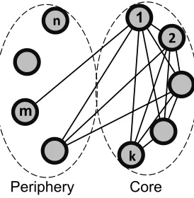
Figure 1: Structure of the efficient network with separable heterogeneous connection model. The connected component has a generalized star structure. n is the number of nodes in the network, m is the number of nodes in the connected component, and k is the number of nodes in the core (complete subgraph). Nodes are sorted according to their costs i.e.

c₁ ≤c₂ ≤ · · · ≤c_n.

2.1

Efficient Structures under Separable Connection Costs

In Lemma 1, we determine the efficient structure for a connected component. Then in Proposition 1, we determine the structure of the efficient network in general.

Lemma 1 If the efficient network with separable cost model is connected then it has a

“gen-eralized star” structure with the following characteristics: (a) All nodes are connected to

node 1 ( the node with minimum connection cost). (b) Nodesi andj (i, j 6= 1) are connected iff b(1)−b(2)> .5(ci+cj).

Proof. Let N represents nodes in the connected network. If there exists a subset of nodes

M ={v1, ..., vm} (M ⊂N) that are not connected to node 1, we show that the network is

not efficient. Since N is connected, there exists a set of links, L = {l1, ..., lm} where li is

adjacent to vi2. Suppose li connects vi to wi (wi 6= 1 by definition). Now, if we remove all lis and connect all vis to node 1, we have reduced the total connection cost of the network

bymc1−

m P

k=1

cvk <0.

Now, to address the benefits, note that we have not changed the number of links; there-fore direct benefits remain the same. Furthermore, the diameter of the new network is 2.

2_{For any subset M ={v}

1,· · · , vm} of a connected network N (M 6≡ N), we can show that there are

Therefore every distance that is not 1 is capped at 2, making the total benefit larger than that of the original network. This results in at improvement in the total utility, indicating that the original network was not efficient.

Furthermore, having established that the maximum distance in the efficient network is no larger than two, every node i and j (i, j 6= 1) are connected iif b(1)−b(2)> .5(ci+cj).

Proposition 1 determines the structure of the efficient network and shows that the efficient network is a spectrum of solutions.

Proposition 1 In the connection model, for a finite set of agents, N ={1, .., n}, if cij =ci

for all i, j ∈ N, where ci ∈ C = {c1, c2, ..., cn} and assuming, c1 < c2 < · · · < cn, the

structure of the efficient network is as follows: Let m be the largest integer between 1 and n

such that 2b(1) + 2(m−2)b(2) >(c_m+c₁). If i > m, then i is isolated. If i≤m, then there is exactly one link between i and 1; also there is one link between i and j (1< i, j ≤m) iff

b(1)−b(2) > .5(ci+cj).

Proof.

First, we show there is at most one connected component in the efficient network. Next, we find the condition for each node to be in the connected component, which has the gener-alized star structure according to Lemma 1.

Assume that the efficient network has more than one (e.g. two) connected components with (mi, ℓi) being respectively the number of nodes and links in connected component i. According to Lemma 1, each connected component has a generalized star structure. The total benefit of each component is B1 = 2ℓ1b(1) + (m1(m1 −1)−2ℓ1)b(2) and B2 =

2ℓ2b(1)+(m2(m2−1)−2ℓ2)b(2) respectively. Supposehandh′are nodes with minimum costs

in component 1 and 2 respectively and without loss of generalitych < ch′. If we disconnect all

links connected toh′ _{and connect them directly toh, total cost decreases by (c}

h′−c_h) per link.

To determine which nodes belong to the connected component, GC, in the efficient

net-work, we define, for node i, Ai , 2b(1) + 2(k −2)b(2)−c1−ci where k is the number of

nodes in the connected componentGC. We show thati is in GC iff Ai ≥0. First, Ai >0 is

the sufficient condition for i to be in GC. This is because connecting i to node 1 increases

the total utility by exactly Ai, as the diameter of GC is at most 2, according to Lemma 1.

Also if A_i < 0, then i will be isolated so A_i ≥ 0 is also the necessary condition. This is because icannot be only connected to 1 since Ai <0, so the only way fori to be connected

is by having more than one link. From Lemma 1, for ito have a link toj 6= 1, we must have

ci+cj <2b(1)−2b(2). But: ci+cj > c1+ci >2b(1) + 2(k−2)b(2)>2b(1)−2b(2), where

we use the fact that cj > c1 and Ai <0, so i cannot have more than one connection either,

thus i will be isolated. Note that Ai >0 also means Aj >0 for all j < i since cj < ci, thus

all lower cost nodes will also be in GC, so the smallest i for which Ai <0 provides the size

of the connected component in the efficient network.

A typical structure for the efficient network with heterogeneous separable cost model is illustrated in Figure 1.

2.2

Characteristics of Networks with Separable Cost Model

2.2.1 Core-Periphery structure

We show that the efficient network has a Core-periphery structure, a widely observed structure in various social and economic networks (i.e. see for example Zhang et al. (2014); Rombach et al. (2014)). We adopt the formal definition from Bramoull´e (2007), which states that a graph g has a core-periphery structure when agents can be partitioned into two sets, the core C and the periphery P, such that all partnerships are formed within the core and no partnership is formed within the periphery. For an efficient network, let k be the largest integer between 2 and n such that b(1)− b(2) > .5(ck−1 +ck). The efficient

a set P = {k + 1, . . . , n} which can only have connections to the complete subgraph. If

b(1) −b(2) > (ck−1 +ck) then k and k−1 are connected and there is also a link between

every nodei, j(i, j ≤k and ci, cj ≤ck), which forms a complete subgraph. Similarly, we can

show that for every i∈P, which is connected to a node j,cj ≤ck and j 6∈P.

2.2.2 Clustering coefficient

Unlike efficient networks with homogeneous cost model whose clustering coefficients are either one (complete graph) or zero (star structure or empty graph), the clustering coefficient of the efficient network with heterogeneous costs covers a wide range. To find a lower bound, we find the minimum global clustering coefficient of all the efficient networks with a given link density and various connection cost values. To this end, we construct a network that does not break the efficiency condition, provided in the previous section, while producing the minimum possible number of triangles for the given density as follows: Starting from an empty graph and node k = 1, we only establish links from node k to every node i > k in ascending order. We repeat this process for k = 1, . . . , p+ 1 until the total number of links reaches ℓ. p is the largest integer such that ℓ = Pp_k=1(n−k) +J, where J is the residual number of links in thep+1 round of incomplete iteration (J < n−p+1). At thek-th iteration, the total number of connected triplets is increased by n−₂k

+2(k−1)(n−k)+ J₂

+2J p. The first term in this equation results from the fact that nodek will act as a local hub with (n−k) new links who provide n−₂k

C_{ef f}min(g, ℓ) = 3×number of triangles

number of connected triplets of nodes = 3× {

Pp

k=1(k−1)(n−k) +pJ}

Pp k=1{

n−k

2

+ 2(k−1)(n−k)}+ J₂

+ 2J p

(2)

Compared to an Erd˝os-R´enyi (ER) random network with the same link density, some algebra reveals that the clustering clustering coefficient of the efficient heterogeneous network exceeds that of an ER network when then number of nodes is greater than 10 and the link density is larger than 4(2_n(nn₋−₁₎5). For sufficiently large networks, the condition simplifies to having link density greater than 8

n.

3

Conclusion

Acknowledgements

This work was supported by DARPA Contract NNA11AB35C. The authors are grateful to Peter Ludlow (Stevens) and Pedram Heydari (UCSD) for insightful comments.

References

Bala, V. and Goyal, S. (1997). Self-organization in communication networks. Technical report, Econometric Institute Research Papers.

Bramoull´e, Y. (2007). Anti-coordination and social interactions. Games and Economic Behavior, 58(1):30–49.

Carayol, N. and Roux, P. (2009). Knowledge flows and the geography of networks: A strategic model of small world formation. Journal of Economic Behavior & Organization, 71(2):414–427.

Galeotti, A., Goyal, S., and Kamphorst, J. (2006). Network formation with heterogeneous players. Games and Economic Behavior, 54(2):353–372.

Goyal, S. (1993). Sustainable communication networks. Econometric Institute, Erasmus University Rotterdam.

Jackson, M. O. et al. (2008). Social and economic networks, volume 3. Princeton University Press Princeton.

Jackson, M. O. and Rogers, B. W. (2005). The economics of small worlds. Journal of the European Economic Association, 3(2-3):617–627.

Jackson, M. O. and Wolinsky, A. (1996). A strategic model of social and economic networks.

Journal of economic theory, 71(1):44–74.

Persitz, D. (2010). Core-periphery r&d collaboration networks. Working paper.

Rombach, M. P., Porter, M. A., Fowler, J. H., and Mucha, P. J. (2014). Core-periphery structure in networks. SIAM Journal on Applied mathematics, 74(1):167–190.

Vandenbossche, J. and Demuynck, T. (2013). Network formation with heterogeneous agents and absolute friction. Computational Economics, 42(1):23–45.