The effect of including the environment in the neoclassical growth model

Munich Personal RePEc Archive

The effect of including the environment

in the neoclassical growth model

Halkos, George and Psarianos, Iacovos

Department of Economics, University of Thessaly

24 November 2015

Laboratory of Operations Research,

Department of Economics, University of Thessaly

This study begins with an exposition of basic principles of the theory of Optimal Control as this is used in the development of the theory of Economic Growth. Then, a brief presentation of the Neoclassical Model of Economic Growth follows and two applications are presented. In the first, optimal control techniques are used, in the context of neoclassical growth, to maximize the representative household’s total intertemporal welfare. In the second, the same problem is posed with two additional variables that affect welfare in opposing ways: and

In both applications, the are derived. This allows for

a preliminary comparison of the resulting under the criterion

of welfare maximization with and without environmental externalities. Finally, using a balanced panel data of 43 countries and for the time period 199002011 we test the validity of including the environment in the neoclassical growth model approximating pollution abatement with the electricity production from renewable sources and pollution with carbon dioxide emissions. With the help of adequate econometric panel data methods we test the validity of the environmental Kuznets curve hypothesis for the full sample, as well as for the OECD and non0OECD countries.

Economic Growth; Physical Capital; Technological Progress; Environment; Pollution.

#$

The relationship between economic growth and the environment has received

much attention recently. The literature considering this relationship is vast. It covers

the theory on growth and natural resources extraction and depletion, explores the

impacts of endogenous growth theory and investigates the link between

environmental pollution and income.

The advancement of economic growth theory started with the Solow0Swan

model (Solow, 1956; Swan, 1956) with exogenous technological progress and growth

being considered either with exogenous saving rates as in the Solow0Swan model or

with households’ consumption and savings optimization models called optimal

growth or Ramsey models (Ramsey, 1928; Cass, 1965; Koopmans, 1965). These

models were followed by endogenous growth models where the “engine of growth” is

either technological progress (Romer, 1990) or human capital accumulation (Lucas,

1988).

Natural resources contribute significantly to production. In the basic form of

the neoclassical growth theory the contribution of natural resources in production is

completely missing. In 1972 the perception of the Solow0Swan model (with three

inputs, namely labor, capital and production methods) was confronted by the report of

the Club of Rome “the Limits to Growth” (Meadows et al., 1972). In the report it was

predicted that the exhaustion of non0renewable resources will result to the fall down

of the global economy and the worldwide collapse of the standards of living.

Specifically, the report notified humanity for the damaging influence of uninterrupted

and rapid economic growth. More pollution and inappropriate use of non0renewable

resources may stop economic growth. The economic growth versus the environment

dispute considered the relationship between growth and quality of the environment

De Bruyn (1992) summarizes the attitudes in this dispute and distinguishes the

radical and conditional supporters together with the weak and strong antagonists.1

Specifically, the radical and conditional supporters of economic growth propose a

direct positive relationship between growth and environmental quality. The former

believe that growth increases technological innovation requiring more R&D and

changes the standards of living resulting in a better quality of the environment. The

latter considers growth as a requirement for environmental management raising funds

necessary for adoption of appropriate environmental policies (Simon, 1981; World

Bank 1992). The weak and strong antagonists consider economic growth as harmful

for the environment. The weak antagonists believe that economic growth is associated

with more output damages the environment. The reduction in growth of specific

polluted economic sectors may be necessary to recover environmental quality (Arrow

at al., 1995). Similarly, strong antagonists claim that in the LR growth will be

damaging the environment and the way out is to decrease economic growth

(Meadows et al., 1972; Daly, 1991).

There are various theories of the relationship between economy and

environment. The classifies this relationship in terms of the irreversible

damage imposed to the environment hitting a threshold ahead of which production is

so defectively influenced that the economy shrinks. The is based on

the idea that pollutants’ emissions are reduced with additional economic growth but

the new pollutants replacing them are raised. In this way the validity of the calculated

turning points is questioned and there is possibility that environmental damage

persists to be enhanced as economies develop (Everett et al., 2010). According to the

international competition first increases environmental damage

up to the point where developed countries begin to decrease their environmental

1

effect but at the same time export activities polluting the environment to poorer

countries. In this way we may end0up in a non0improving situation. Finally, the

considers economic growth and the environment as a false

dichotomy. It finds that effective environmental policies may raise the level of R&D

into more resource efficient processes, leading to higher competitiveness and

profitability (Everett et al., 2010).

Empirical findings of the relationship between economic growth and the

environment and the investigation of the environmental Kuznets curve hypothesis are

based on model specifications. The environmental Kuznets curve (EKC) hypothesis

suggests the existence of an inverted U0shape relationship between environmental

damage and per0capita income. Specifically, it relates environment (using

environmental pollution or damage as dependent variable) with economic

development represented by economic variables (like GDP/c in level, square and

cubic values as independent variables). Depending on data availability different

variables have been used to approximate environmental damage like air pollutants

(SOX, NOX, CO2, PM10, etc.), water pollutants (e.g. toxic chemicals discharged in

water, etc.) and other indicators like deforestation, municipal waste, energy use and

access to safe drinking water.

This paper is structured as follows. Section 2 discusses the existing theoretical

and empirical literature. Sections 3 and 4 present the dynamic models of modern

macroeconomic theory together with two applications with the second one referring

to the proposed theoretical inclusion of the environment into the neoclassical growth

theory.2 Section 5 presents data and econometric methods used in the proposed

application and the related empirical findings. The final section concludes the paper.

2

%$

Reviews and critiques of the EKC studies may be found among others in Arrow

. (1995), Ekins (1997), Ansuategi . (1998), Stern (1998) and Halkos and

Tsionas (2001). The differences in the extracted relationships and in the calculated

turning points may be justified by the econometric models’ specification and the

adoption of static or dynamic analysis (Halkos, 2003). Simultaneously, the addition of

more explanatory variables in the model specification influences the estimated

relationship. Roca et al. (2001) claim that estimated EKC is weaker when using more

independent variables apart from income. Empirical evidence is unclear and mixed

(Galeotti et al., 2006; He and Richard, 2010; Chuku, 2011).

Various studies have ended up to linear and monotonic relationships between

damage and income.3 Akbostanci et al. (2009) and Fodha and Zaghdoud (2010)

considering the link between income and environment in Turkey and Tunisia

respectively, find a monotonically increasing relationship between CO2 emissions and

income. Others have found inverted0U shaped relationships with turning points

ranging from higher than $800 to less than $80,000, implying a feasible division of

environmental damage from economic growth (Grossman and Krueger, 1995; Holtz0

Eakin and Selden 1995; Panayotou 1993, 1997; Cole et al., 1997; Stern and Common

2001; Halkos, 2003; Galeotti et al., 2006). He and Richard (2010) for the relationship

between CO2 emissions and GDP in the case of Canada and by using parametric,

semi0parametric and non0linear models found weak evidence of the EKC hypothesis.

Stern (1996) claim that the mix of effluent has shifted from sulphur and NOX

to CO2 and solid waste, in a way that aggregate waste is still high and even if per unit

output waste has declined, per capita waste may not have declined. Regressing per

capita energy consumption on income and temperature gave them an inverted U0

3

shape relationship between energy and income. Energy consumption peaked at

$14600. The authors claim that the results depend on the income measure used. If

income in PPP is used, the coefficient on squared income was positive but small and

insignificant. If income per capita was measured using official exchange rates, the

fitted energy income relationship was an inverted U0shape with energy use peaking at

income $23900.

Other researchers have found shape relationships (Friedl and Getzner, 2003;

Martinez0Zarzoso and Bengochea0Marancho, 2004; Akbostanci et al., 2009; Halkos,

2012) showing that pollution and the associated environmental damage from

economic growth may be a temporary phenomenon (He and Richard, 2010).

Grossman and Krueger (1995) and Shafik and Bandyopadhyay (1992) claim that at

high0income levels, material use increases in such a way that forms an N0shape

relationship.

&$ ' (

The models of modern Macroeconomic Theory – and the models of

Growth Theory in particular – are concerned with the behavior of aggregate economy

through time. In this context, the pattern of private consumption is summarized in,

and by, the behavior of the so0called or

Most usually, the consumer is assumed to face an indefinitely large or

‘infinite’ time horizon and needs to determine all per0period consumption

expenditures for this horizon.4 From each period’s expenditures the consumer derives

a certain level of satisfaction or The consumer’s objective is to achieve an

) *) which, under given constraints,

* + the of the ) ,) . This total

utility is generally expressed by the

4

(

)

0

, ,

ρ

∞ ₋ =

=

∫

d

₍₁₎

where is per capita consumption at time , is per capita (per worker)5 physical

capital at time , and is simply the ‘time variable’.6

The typical problem of maximizing intertemporal utility is essentially an

problem which can be stated as

(

)

0

max

max

∞ −ρ

, ,

=

=

∫

d

₍₂₎

with constraints

(

, ,

)

≡ =

i (3)

0 0

=

=

(4)

lim

(

−ρ

)

0

→∞

≥

(5)

At this point, we note that all variables depend on time and simplify notation by

omitting time subscripts whenever time dependence is easily understood. Further,

one may discern the following elements.

1. Function

( )

⋅ which is called and measures

consumer’s per0period utility. A common in growth models instantaneous utility

function is

( )

1

1

0,

1

1

σ

σ

σ

σ

−

−

=

>

≠

−

where

σ

is the inverse of the elasticity of intertemporal substitution in consumption7,

and

! "

# _{" $ % &}

2. Function

( )

⋅ which depicts per capita investment. The quantity of per capita

physical capital evolves through time according to this equation and influences the

future productive capacity of the economy. In optimal control theory (differential)

equation (3) is often referred to as !

3. ‘Variable’ , is in actuality a $ As it is evident from the statement

of the problem, is the ‘variable’ with respect to which the objective function is

maximized.8 This is why is referred to as the or

In addition, we note that control variable affects the objective function in two

ways: First directly, with its own value and second indirectly, by influencing the

value of variable that also enters the objective function.

4. ‘Variable’ which evolves as a function of time according to differential

equation (3). The value of determines at any time the state of the dynamical

system under examination. For this, is known as the

5. Parameter

ρ

>0, which expresses the " In other

words,

ρ

is a based on which the values of future flows of utility are

converted into terms.

6. Condition (4) which states that the initial value of during period =0 is equal

to ₀.

7. Condition (5) which states that at the end of the problem’s time horizon the

quantity of per0capita physical capital cannot be negative.

For the solution of the problem given in relations (2)–(5), we form the function

known as

(

, ,

)

(

, ,

)

ρ

λ

−

=

+

(6)

) _& σ _{* +}

As its name implies, equation (6) measures units of utility expressed in present value

terms (time period 0). The new term in equation (6) is the ‘variable’

λ

. This term

(also a function of time) is called the It measures the

that will be generated by an additional unit of per capita physical

capital at time , when this value is expressed in units of utility of the initial time

period (time 0).9

Necessary conditions for optimization are

0

∂

=

∂

(7)

λ

∂

= −

∂

i

(8)

όπου

λ

≡

λ

i d

d .

λ

∂

=

∂

i

(9)

(

)

lim

λ

0

→∞

=

(10)

Equation (10) is known as and is necessary for optimality, as

it precludes the possibility of 10 It ensures that as we approach

at the end of the problem’s horizon it must be either =0, or

λ

=0. The essence

of this condition is that either no quantity of physical capital exists, or that any

remaining quantity offers zero utility in present value terms (expressed in units of

utility at time =0).

. _& λ

/0 ₁

Typically, it is preferable for further analysis to obtain the solution of the

problem as a system of differential equations.11 Aiming at that, we write

as

(

, ,

)

(

, ,

)

ρ ρ

λ

−





=



+



(11)

Next we define the as

ρ

which yields

( )

,

(

, ,

)

=

+

(12)

Note that = ρ

λ

is the of . It measures the value

of extra units of utility that will be generated by an additional unit of per capita

physical capital at time , when this value is expressed in units of utility at time

. The first0order conditions now become

∂

=

0

∂

(13)

ρ

∂

=

−

∂

i

(14)

∂

=

∂

i

(15)

(

)

lim

λ

lim

−ρ

0

→∞

=

→∞

=

(16)

Notice that the right side of (16) implies that the current value of an additional unit of

, that is , must be either finite or grow at a rate less than

ρ

>0, so that the

discount factor −ρ confines the present value of to zero.

Now, a useful extension would be to assume that population increases at a

constant exogenous rate

γ

_{{ }#} ≡ >0. This implies that # =#₀ where all

symbols have the usual meaning. Based on the above, one can write the optimization

problem as

( )

( )

₀

0 0

max

∞ −ρ

,

#

max

∞ −ρ

,

#

=

=

=

∫

d

∫

d

≃

( )

( )

0

max

∞ − −ρ

,

=

∫

≃

d

(17)

This change does not alter the optimality conditions as the final expression in (17)

results from the original after dividing by the constant#₀. The latter is initial

population size (period =0), which with appropriate $ can be set

equal to one.

The important new element is that the discount rate of the modified problem,

0

ρ

− > , is smaller by compared to the original. As a result, with an increasing

population it is desirable that present generations reduce the rate at which they

convert future utility values into equivalent current ones.12 Such a decision will

enable higher savings/investments for the creation of new units of physical capital to

be used by future generations. Finally, note that the current value shadow price of

is equal to = (ρ− )

λ

. Conditions (13) and (15) remain the same, while

conditions (14) and (16) become

(

ρ

)

∂

=

−

−

∂

i

(18)

and

lim

(

λ

)

lim

− −(ρ )

0

→∞

=

→∞

=

(19)

Now, observe that the right side of (19) implies that the current value of an additional

unit of , must be either finite or grow at a rate less than

ρ

− >0. In such case,

the discount factor − −(ρ ) would restrict the present value of to zero.

-$ . ( / 0

The neoclassical model has been a cornerstone for the development of modern

economic growth theory. It is founded on two basic equations:

and ! The production function

describes the way or can be combined to

produce the economy’s final output.13 Factors of production are grouped in two

broad categories: % #, and % &. The latter includes tools,

machinery, and facilities (plant and equipment) used in production.14 The production

function is of ' ( form with Constant Returns to Scale (CRS). Denoting

total output by ), it is

(

)

1

,

,

0

1

)

≡

* # &

=

# &

α −α

< <

α

(20)

The labor force, #, coincides with population which is, at present, constant.

Note that the production function (20), satisfies the principle of

% as it is

( )

( )

₁1

0,

( )

2 ₂

( )

(

1

₂

)

1

0

# ##

*

&

*

&

*

*

#

#

#

#

α α

α α

α

α

α

− −

− −

∂

∂

−

≡

=

>

≡

= −

<

∂

∂

i

i

i

i

and

( )

( ) (

1

)

0,

( )

2

( )

₂

(

1

₁

)

0

& &&

*

#

*

#

*

*

&

&

&

&

α α

α α

α

α

α

+

∂

−

∂

−

≡

=

>

≡

= −

<

∂

∂

i

i

i

i

/4 _{& 1 " " ! /}

" "

" * 5 +

Also, the same function abides to the known as+

( )

( )

( )

( )

0 0

lim

lim

and

lim

lim

0

# & # &

*

*

*

*

#

&

#

&

→ → →∞ →∞

∂

∂

∂

∂

=

= ∞

=

=

∂

∂

∂

∂

i

i

i

i

Finally, it is* #

(

,0

)

=*

(

0,&

)

=0, meaning that production of positive output

necessitates the use of positive amounts from both inputs.

The second fundamental equation of the neoclassical model is

,

0

1

&

i

= −

)

#

−

δ

&

< <

δ

(21)

and describes how physical capital accumulates. The term on the left side of (21) is

equivalent to the difference &₊ −& in % that is, when the interval

between time periods + and is arbitrarily small (close to zero). Generalizing, a

‘dot’ over any variable (of time) such as &, stands for the first derivative of this

variable with respect to time,

0

lim

&

&

&

,

0

&

+

→

−

≡

≡

>

i

d

d

and measures the of & in $ The term

) − # on the right side of (21), is People spend on

consumption a total amount equal to #, where is per capita consumption,

whereas they save a value equal to )− #. The latter amount – total savings – is in

turn invested in the production of new units of physical capital.15 Finally, the term

&

δ

measures the ‘wear and tear’ of physical capital during production. The

assumption here is that a fixed proportion,

δ

, 0< <

δ

1, of the existing quantity of

physical capital in every period. Evidently, the aggregate quantity of

physical capital, &, increases when ) − #>

δ

& , decreases if )− #<

δ

&, and

remains the same when ) − #=

δ

& .16

, -. / $ ' + 0

1 /

In this section, the steady state (dynamic long0run equilibrium)

of the standard neoclassical growth model is presented. Optimality is ensured by the

theoretical contrivance of an ideal who is assumed to run the economy

with objective to maximize the present value of the representative agent’s total

intertemporal utility.17 This will later permit us to better understand the possible

growth0effect of enriching the neoclassical model with issues related to the

environment.

The following equations (22)–(24) set the model as

(

)

1

,

)

=

* # &

=

# &

α −α (22)

1

&

i

=

# &

α −α

−

#

−

δ

&

(23)

{ }

0 #

#

=

#

⇒

#

i

=

#

⇒

γ

=

(24)

where _{{ }2} 2

2

γ

≡

i

denotes the growth rate of any variable (of time) 2 . Equation (25)

poses the maximization problem

( )

( )

( ) 1

0 0

1

max

max

1

σ

ρ ρ

σ

−

∞ _{− −} ∞ _{− −}

= =

−

=

−

∫

d

∫

d

₍₂₅₎

Equation (26) presents the current0value Hamiltonian

/#

/) _{" 7}

" 8

(

)

1

1

1

1

&

# &

#

&

σ

α α

δ

σ

− −

−

=

+

−

−

−

(26)

Equations (27)0(29) invoke the necessary conditions

0

−σ _&

#

∂

= ⇒

=

∂

(27)

(

)

_{& & &}

#

(

1

)

&

(

)

_{& &}

&

α α

ρ

α

−

δ

ρ

∂





=

−

−

⇒



−

−



=

−

−

⇒

∂

i i

{ }&

*

&

( )

γ

ρ

δ

⇒

= − + −

i

(28)

1

& &

&

# &

α −α

#

δ

&

∂

∂

=

⇒

=

−

−

∂

∂

i

(29)

Differentiation with respect to time of the logarithm of (27) yields

{ } { }&

σγ

γ

−

=

+

(30)

Equating (28) and (30) results in

{ }

*

&

( )

{ }

#

(

1

)

&

α α

ρ δ

α

ρ δ

γ

γ

σ

σ

−

− −

−

− −

=

i

⇒

=

(31)

On the other hand it is known that

{ }2 { }

γ

=

γ

+

(32)

for 2 = #, that is, aggregates grow at a rate higher by in comparison to their

respective per0capita magnitudes. Then, from (23) we may write

{ }& { } { }

'

'

# &

# &

&

&

α α α α

γ

=

γ

+ =

−

−

−

δ

⇒

=

−

− − −

δ

γ

(33)

But from (31) it is

{ }

(

1

)

&

#

α

α

σγ

ρ δ

α

−

=

+ +

−

(34)

{ }

{ }

1

'

&

σγ

ρ δ

δ

γ

α

+ +

=

− − −

−

(35)

which is constant as both

γ

_{{ }} and

γ

_{{ }} are constant by definition of steady state.

The fact that the ratio ' #

& = # = is constant implies

{ } { }

γ

=

γ

(36)

Further, since /

/

& & #

) = ) # = is constant, it is

{ } { }

γ

=

γ

(37)

Taking (36) and (37) into account we may write

{ } { } { }

γ

=

γ

=

γ

(38)

Now, note that

γ

_{{ }#} = >0 and log0differentiate (34) to find

{ }& { }# { }&

αγ

αγ

γ

−

= −

⇒

=

(39)

But it is clear from (32) and (38) that

{ }) { }& { }'

γ

=

γ

=

γ

(40)

Then, combine equations (39) and (40) to show that in steady state this economy

grows at a rate equal to the rate of growth of population

{ }) { }& { }'

γ

=

γ

=

γ

=

(41)

Finally, from equations (32), (38) and (41) we conclude that per0capita variables ,

and display zero growth in steady state.

{ } { } { }

0

γ

=

γ

=

γ

=

(42)

Positive growth in per capita variables can be achieved in the neoclassical model by

(

) ( )

1

,

,

0

1

)

=

* ,# &

=

,#

α

&

−α

< <

α

(43)

where , is an index measuring the current level of technology.18

Observe that the as represented here by the

,, multiplies the available quantity of labor and results in

% # . In such a way technological progress increases labor productivity and

makes it possible to produce larger quantities of output using the same aggregate

amounts of labor #, and physical capital, &. Technological progress creates new

productive knowledge at an exogenous rate , that is,

{ }

0 ,

,

=

,

⇒

,

i

=

,

⇒

γ

=

(44)

where ,₀ denotes the initial level of technology (period =0).

To account for technological change, we express variables in units of efficient

labor # This implies that the discount factor must now incorporate increases not

only in population, but also in the quantity of efficient labor. We can easily see that

the appropriate discount factor in the present case is

ρ

− − >0, instead of

0

ρ

− > in the presence of population increases, and simply

ρ

>0 in the original

model. The impact of technological progress is clarified by working out the new

optimization problem for the model expressed in units of efficient labor. This is

achieved by dividing all aggregate variables (functions of time) by the quantity of

efficient labor,#. Thus, we obtain the following: (subscripts denote ‘per unit of

efficient of labor’.) Production per Unit of Efficient Labor

( )

1−α

=

=

(45)

Accumulation of Physical Capital per Unit of Efficient Labor

(

)

1−α

δ

=

−

−

+ +

i

(46)

Maximization of Intertemporal Utility per Unit of Efficient Labor

( )

( )

0 0

0 0

max

∞ −ρ

# ,

max

∞ −ρ

#

,

=

=

=

∫

d

∫

d

≃

( )

( )

( ) 1

0 0

1

max

max

1

σ ρ ρ

σ

− ∞ _{− − −} ∞ _{− − −} = =

−

=

−

∫

∫

≃

d

d

(47)

Current0Value0Hamiltonian

(

)

1 1

1

1

σ α

δ

σ

− −

−

=

+

−

−

−

−

−

(48) Necessary Conditions

0

−σ

∂

= ⇒

=

∂

(49)

(

ρ

)

∂

=

− −

−

⇒

∂

i

(

1

α

)

−α

δ

(

ρ

)





⇒



−

− − −



=

− −

−

i

⇒

{ }

( )

γ

ρ δ

′

⇒

= + −

(50)

where ′

( )

≡ ∂

( )

∂ .

1−α

δ

∂

∂

=

⇒

=

−

−

−

−

∂

∂

i

(51)

Going through the algebra as before, we find that all variables expressed in ‘per

unit of efficient labor’ terms grow in steady state

{ } { } { }

0

γ

=

γ

=

γ

=

(52)

{ } { }

γ

=

γ

+

(53)

where = ,. According to expression (53) per capita variables grow at a rate

higher by (the rate of technological progress) compared to the respective ‘per unit

of efficient labor’ variables. Thus, relations (52) and (53) lead to

{ } { } { }

γ

=

γ

=

γ

=

(54)

Finally, note that

{ }2 { }

γ

=

γ

+

(55)

where 2 = #. Expression (55) states that aggregate variables grow at a rate higher

by in comparison to the respective per capita magnitudes (and at a rate higher by

+ in comparison to the respective ‘per unit of efficient labor’ quantities.) Given

expressions (54) and (55), we conclude that it is

{ }) { }& { }'

γ

=

γ

=

γ

= +

(56)

, 3. / $ ' +

1 /

In this section the 4 is introduced in the neoclassical growth model.

It is assumed that environmental deterioration in the form of is created by,

and associated with, the use of physical capital in production of the final good. No

doubt, this has a negative impact on peoples’ welfare. At the same time, it is also

assumed that pollution can be reduced by devoting part of aggregate output to

the two variables just mentioned: the economy’s aggregate stock of physical capital

0

& > , and the level of ‘Abatement’ 5 >0, both at time .19

(

& 5

,

)

&

5





≡

= 







(57)

It is clear from equation (57) that the level of pollution is increasing with the

aggregate quantity of physical capital and decreasing with expenditures (amount of

resources used) on pollution abatement:

0 0

& 5

& 5

∂ ∂

≡ > ≡ <

∂ and ∂ (58)

To ensure that the present model is consistent with a , or

% where all variables grow at – not necessarily equal – rates, the

restriction is imposed that function

( )

_i is 1 2+ 3.20 In

addition, per0capita consumption and the level of pollution enter the instantaneous

utility function as as in the following equation

(

,

)

1 (1 )

1

,

0,

1

1

ϑ σ σ

σ

σ

σ

− −

−

−

=

>

≠

−

(59)

where

ϑ

>0 stands as a weight of pollution on utility.

Rewriting for convenience the model in aggregate terms one obtains the

aggregate production function

(

)

1

,

)

=

* # &

=

# &

α −α (60)

and the equation of physical capital accumulation

1

&

i

=

# &

α −α

−

#

−

δ

&

−

5

(61)

/. _{7 "}

Equation (61) also represents the economy’s resource constraint asserting that total

output, ) =# &α 1−α, can be allocated into total consumption, '= #, total gross

investment in physical capital,&i +

δ

&, and pollution abatement activities, 5.

Population again grows at a constant exogenous rate

{ }

0 #

#

=

#

⇒

#

i

=

#

⇒

γ

=

(62)

Dividing all aggregate variables by population we express the model in per capita

terms as

( )

1−α

=

=

(63)

(

)

1−α

δ

=

− −

+

−

i

(64)

As regards the pollution level it is

&

&

#

5

5

#

≡

=

=

(65)

that is, total pollution is given by the constant ratio of physical capital to pollution

abatement expenditures both in per0capita terms. Based on (65) the instantaneous

utility function (59) becomes a function of per0capita consumption and per0capita

expenditures on pollution abatement

(

)

( )

(1 )

1

1

,

,

,

0,

1

1

ϑ σ σ

σ

σ

σ

− −

−

 

−

 

 

≡

=

>

≠

−

(66)

Next, note that

ϑ

and

(

1−

σ

)

are constant and %

bundles of goods. Then, the instantaneous utility function (66) can equivalently be

written as

(

,

)

log

(

,

)

log

log

6

≡

=

−

ϑ

or, using (65)

(

,

)

(

, ,

)

log

log

6

≡

6

=

−

ϑ

 

 

 

(67)

Similarly to the previous section, the optimization problem is

( )

0 ,

max

∞ − −ρ

log

ϑ

log

=



−

 



 



 







∫

d

₍₆₈₎

and the respective current0value Hamiltonian becomes

( )

(

)

log

ϑ

log 

δ

= − _{ }+ _ − − + − _

  (69)

Proceeding in the usual fashion, the necessary conditions

0

∂

=

∂

(70)

0

∂

=

∂

(71)

(

ρ

)

∂

=

−

−

∂

i

(72)

along with i =0 and the standard steady0state conditions of the neoclassical model

0

= = =

i i i

, yield

( )

ρ δ

′

= + +

(73)

where ′

( )

is the marginal product of per0capita physical capital. It is now

straightforward to compare with the steady0state condition of the original model

( )

ρ δ

′

= +

(74)

Clearly, the marginal product of in steady state is higher in the model that

takes into account environmental effects.21 As a result, and due to the concavity of

per0capita production

( )

= 1−α, condition (73) implies a steady state with smaller

quantity of per0capita physical capital than (74). Thus, it is optimal for the economy

to accumulate less physical capital than in the model without environmental effects.

The reason is that physical capital is accompanied by the external (social) cost of

pollution. This cost can be compensated in equilibrium by a higher marginal return

of physical capital in production, which is possible only at a lower quantity of the said

factor. As an end result, a lower level of per0capita output (income) is produced as

fewer resources are put in the accumulation of physical capital while part of output is

devoted to environmental protection. In terms of consumers’ intertemporal utility one

may suggest that, in a sense, what is lost because of lower per0capita consumption is

returned thanks to improved environmental quality.

4$ ) ))

7 - (

Using a sample of 43 countries with a full set of data for the variables of

interest we explore the relationship between pollution in the form of carbon dioxide

emissions, economic growth expressed by the gross domestic product and abatement

approximated by the use of renewable energy sources in the production of

electricity22 in the full sample of countries considered (n=43) as well as for the OECD

(n=21) and non0OECD (n=22) countries for the time period 199002011.23

21

7 *)4+ * + 1

1

22

Another variable of interest for our purpose was the 81 19

Specifically, carbon dioxide emissions per capita (CO2/c in kt) stem from

burning of fossil fuels and manufacture of cement and they comprise CO2 produced

throughout the consumption of solid, liquid, and gas fuels and gas flaring. Gross

Domestic Product per capita GDP/c (in current US$) is the sum of gross value added

resident producers plus product taxes minus subsidies (not included in products’

value). Deductions for depreciation of fabricated assets or degradation of natural

resources are not considered.24 Finally, renewable energy sources in the production of

electricity (REN/c) represents electricity production per capita from renewable

sources, excluding hydroelectric, including geothermal, solar, tides, wind, biomass,

and biofuels.25

7 3 4

The basic specification of the model to be estimated may be expressed as:

0

) = +β 2 β α γ ε+ + + (75)

where Yit is the dependent variable and Xit is a k0vector of independent variables.

Stochastic error terms are noted as εit for i=1,2,…M cross0sectional units in periods

t=1,2,…T. Parameters β0, αi and γt correspond to the overall constant of the model

and to cross0section and period specific effects (random or fixed) respectively.

Countries are indexed by i and time by t.

The above equation has been estimated by various panel data methods. First the

fixed effects (FE) method was applied permitting each country to have a different

attributable to forest and land0use change activities. Due to many missing values this variable was omitted from our analysis.

23

The full sample database used has 946 observations per variable. The countries used are the following:

0 "' 2 5%#3: Australia, Austria, Canada, Chile, Denmark, Finland, France, Greece, Ireland, Italy, Japan, Korea, Luxembourg, Mexico, Netherlands, Norway, Portugal, Sweden, Turkey, UK, USA

. ,0 "' 2 5%%3: Argentina, Bolivia, Brazil, China, Colombia, Costa Rica, Caribbean, Cuba, Dominikan Rep, Gabon, Guatemala, Indonesia, Nicaragua, Panama, Peru, Philippines, Senegal, Singapore, El Salvador, Thailand, Trinidat and Tobaco, Uruguay.

24

For more details see http://data.worldbank.org/indicator/NY.GNP.PCAP.CD

25

The source of data is IEA Statistics © OECD/IEA 2012 (http://www.iea.org/stats/index.asp), subject

intercept and treating αi and γt as regression parameters. Then the random effects (RE)

method was employed where individual effects are treated as random. That is αi and γt

are treated as components of the random disturbances. If country and time effects are

correlated with the independent variables then RE model cannot be consistently

estimated (Hsiao, 1986, Mundlak, 1978). Both FE and RE are inefficient in the

presence of heteroskedasticity (Baltagi, 2001). To tackle heteroskedasticity and

possible patterns of correlation in the residuals, Generalized Least Squares (GLS)

specifications are used and the parameters estimation of GLS is given as:

1 1 1

ˆ _{(2 )}

β _{= ′Φ Χ Χ Φ Υ}− − _′ −

(76)

Since the panel data employed in this study includes large N and T dimensions,

non0stationarity should be explicitly considered and the dynamic misspecification of

the pollutants' equations should be addressed, as pointed0out by Halkos (2003). If we

base our analysis on a static model, then adjustments to any shock result in the same

period in which these occur, but this could only be justified in equilibrium or if the

adjustment process is fast. According to Perman and Stern (1999) this is unlikely to

be the case and on the other hand, it is expected that the adjustment to long0run

equilibrium emission levels is a particularly slow process.

An additional econometric concern for estimating the model is the potential

bias occurring from the possible endogeneity between the renewable energy variable

and CO2/c emissions, since the use of renewables is expected to be greater in

countries where air pollution is extensive.

To address the aforementioned concerns we employ the Arellano and Bond

(1998) Generalized Method of Moments (A0B GMM). GMM controls for the

endogeneity that is likely to exist in the determination of the dependent variables and

predetermined variables as instruments in a systematic way. Since there is evidence

of heteroskedasticity we use the more relevant two0step Arellano–Bond procedure.

Moreover, we report Orthogonal0Deviations GMM to control for fixed country

effects.

To be more specific, we have used the GMM with its estimators relying on

moments of the form

( )

( )

( )

1 1

β β β

= =

′ ′

=

∑

=

∑

Ψ (77)

With Ψ being a ; matrix of instruments for cross section and

( )

β =

(

) −

(

2 ,β

)

)

. GMM minimizes the following quadratic form with respect

to β

( )

( )

( )

( )

( )

1 1

/ β β 6 β ζ β 6ζ β

= =

 _′   _′  _′

=_ Ψ _{ } Ψ _=



∑

 

∑

 (78)

With 6being a weighting matrix. Orthogonal deviations state each observation

in the form of deviations from the average of future sample observations and each

deviation is weighted in such a way as to standardize variance (Arellano, 1988). That

is:

* =

[

−( ₍ +1₎+ +... _;) / (;− )

]

(;− ) / ;− +1 t=1,…T01 (79)

The (Ti –q) equations for unit i can be expressed as

) =δ + η + (80)

with δ being a parameter vector, wi a data matrix with the time series of lagged

endogenous variables, the x' s, and time dummies and di a (Ti0q) x1 vector of ones.

Linear GMM estimators of δ may be calculated as (Arellano and Bond, 1998)

(

)

      _′ ′ Ν       ′             ′ ′ Ν       ′ =

∑

∑

∑

∑

∑

∑

− ) < < < < < < <

< * 1 * *

* 1 1 . . 1 1 .

where and some transformation of wi and Yi like first differences and

orthogonal deviations. Zi and Hi are the instrumental variables and individual specific

weighting matrices respectively.

Our initial model was a general dynamic model with the dependent and the

independent variables lagged p and q times. Based on likelihood criteria (like the

Akaike and Bayesian Information criteria) and omitting the insignificant dynamics we

ended up to an autoregressive distributed lag model of AD(1,0). To specify how a

country adjusts to the long0run equilibrium level of emissions a partial adjustment

model was assumed of the form

*

2 2

2 1 2 1

( / ) ( / )

( / ) ( / )

'= '=

'= '=

κ

− −

 

=  

  (82)

Where (CO2/c)t, (CO2/c)t01 and (CO2/c)t* are the actual, the lagged by one period and

the desired levels of emissions respectively and κ the adjustment coefficient

(0<κ<1).26

Box0Cox tests were used to establish the relationship to test linearity against

logarithmic specification forms between the variables of interest and our tests indicate

the following specification:

(CO2/c)it = β0 + αi + γt + β₁(GDP/c)it + β₂(GDP/c) 2

it + β3(GDP/c) 3

it +

+ β₄REN/c + β5(CO2/c)i,t01 + εit (83)

where "0%6 is carbon dioxide emissions per capita, GDP/c is per capita Gross

Domestic Product and REN/c the electricity production per capita from renewable

sources.

Various tests and diagnostics are used. The Hausman test compares the slope

parameters estimated by the fixed and random effects models considering the

26

inconsistency of the random effects model estimates. Rejection of the null hypothesis

implies that the random effects model is inconsistently estimated and if there are no

other econometric problems the fixed effects model should be used. Testing for cross0

sectional dependence the Pesaran’s (2004) cross0section dependence (CD) test is

applied to estimate if the time series in the panel considered are cross0sectional

independent.27 The test is valid for large N and T in any order and is robust to

structural breaks (Camarero et al., 2011). Moreover, a Breusch0Pagan LM test for

individual effects for the random effects estimation robust standard errors is applied.

To examine the stochastic properties of the variables under consideration

various unit root tests are usable (Levin, Lin and Chu, 2002; Harris and Tzavalis,

1999; Hadri, 2000; Breitung, 2000; Breitung and Das, 2005; Im, Pesaran and Shin,

2003;28 and Fisher type29 tests). The Levin–Lin–Chu, Harris and Tzavalis, and

Breitung tests make the simplifying assumption that all panels share the same

autoregressive parameter so that ρi = ρ for all i (∀i). The other tests however, allow

the autoregressive parameter to be panel specific. Imposing the restriction that ρi = ρ

∀i implies that the rate of convergence would be the same for all countries, an

implication that is too restrictive in practice. On the other hand, the Im, Pesaran and

Shin test allows for heterogeneous panels with serially uncorrelated errors but

assumes that the number of time periods, T, is fixed. Fisher type tests allow for large

T and finite or infinite N and are suitable in our case. Moreover, except for the Fisher

tests, all the other tests require that there be no gaps in any panel’s series.

Finally, panel co0integration tests are used. Pedroni (1999, 2000, 2004)

proposed seven test statistics for the null of no co0integration; specifically, four panel

27

STATA’s “xtcsd” command was used (De Hoyos and Sarafidis, 2006).

28

Im, Pesaran and Shin (2003) test is generally more powerful than the Fisher type and that proposed by Levin, Lin and Chu (2002) tests (Barbieri, 2006).

29

* tests are based on combining the p0values of the N cross0sectional tests rather than using

statistics and three group statistics testing either panel co0integration or cointegration

across cross0sections.

7 > 4

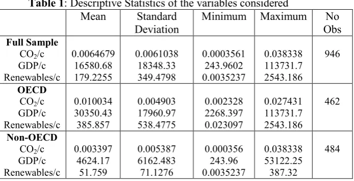
Table 1 and Figure 1 present the descriptive statistics and the graphical

presentation of the variables of interest respectively. Similarly, Table 2a presents

some of the panel unit root tests for the variables under consideration. Graphical

examinations indicate that both a trend and a constant term were to be included in the

model formulation. The number of lags was determined using the Akaike and

Schwarz information criteria. Looking at Table 2a we see support against non0

stationarity in levels with our variables being I(1) implying that they are stationary in

first differences and non0stationary in levels. Table 2b presents the Pedroni

Cointegration tests where in four of the seven cases we reject the null hypothesis of

no cointegration at the conventional statistical significance levels.

In the static model according to the Hausman test, FE is preferable to RE for

the full sample, while RE estimates are preferable in the case of the non0OECD and

OECD sub0samples. Based on the estimates of the static model, the extended use of

renewable energy sources has a significantly negative direct effect on CO2/c

emissions. This effect is robust even after controlling for the income level and is

consistent in all specifications examined.

#: Descriptive Statistics of the variables considered Mean Standard

Deviation

Minimum Maximum No Obs

7 8 )

CO2/c

GDP/c Renewables/c 0.0064679 16580.68 179.2255 0.0061038 18348.33 349.4798 0.0003561 243.9602 0.0035237 0.038338 113731.7 2543.186 946 0 "'

CO2/c

GDP/c Renewables/c 0.010034 30350.43 385.857 0.004903 17960.97 538.4775 0.002328 2268.397 0.023097 0.027431 113731.7 2543.186 462

. ,0 "'

CO2/c

[image:30.595.83.430.610.787.2]

7 #: Basic graphical presentation of the variables of interest 7 )

!

"

. ,0 "' 0 "'

!

"

# $ $

!

"

% : Summary of panel unit root tests (H0: Panels contain unit roots)

! + % %

0 6

,(* * !

* !

7 '

+ % % 0 6

,(* * !

* !

0.9091 0.1129 0.4705 0.0000 0.0000 0.0000

0.9828 0.1274 0.4599 0.0000 0.0000 0.0000

CO2/c

0.9837 0.8586 0.4189

dCO2/c

0.0000 0.0000 0.0000

1.0000 0.9986 1.0000 0.0000 0.0000 0.0000

0.4397 0.6798 0.9999 0.0000 0.0000 0.0000

GDP/c

1.0000 1.0000 1.0000

dGDP/c

0.0007 0.0007 0.0000

1.0000 0.9835 1.0000 0.0000 0.0000 0.0000

0.3058 0.1345 1.0000 0.0000 0.0000 0.0000

GDP/c2

1.0000 1.0000 1.0000

dGDP/c2

0.0745 0.0002 0.0000

1.0000 0.2734 1.0000 0.0000 0.0000 0.0000

0.0005 0.0005 1.0000 0.0000 0.0000 0.0000

GDP/c3

1.0000 1.0000 1.0000

dGDP/c3

0.7658 0.0000 0.0000

1.0000 0.3272 0.8191 0.0000 0.0000 0.0000

1.0000 0.9879 0.9999 0.0002 0.0000 0.0000

RENEW/c

1.0000 0.8423 0.0655

d(RENE/c)

0.0012 0.0000 0.0000

% : Pedroni cointegration test (H0: No cointegration) (deterministic intercept and trend)

To tackle the various concerns mentioned in the previous sub0section we use

the A0B GMM. The significance of the lagged dependent variable (p0value = 0.000)

suggests that dynamic specifications should be preferred.30 It should be noted that the

assumption of uncorrelated errors is important here, so tests for first0 and second0

order serial correlation related to the residuals from the estimated equation are

reported in the last columns. These tests are asymptotically0distributed as normal

variables under the null hypothesis of no0serial correlation. The test for AR(1) is

rejected as expected, while there is no evidence that the assumption of serially

uncorrelated errors is inappropriate in all significance levels. For all specifications we

test the validity of instruments with the Hansen test, which failed to reject the null

that the instrumental variables are uncorrelated with the residuals. The reported J0

statistic is related to the Sargan statistic and the value of the GMM objective function

at the estimated parameters while the Wald χ2 test strongly rejects the null hypothesis

(of all coefficients being zero).

Columns 406 in Table 3 report GMM Orthogonal0Deviations estimates of the

pollution equation. Taking into account endogeneity in the A0B GMM estimates the

effect of renewable energy sources on CO2/c emissions remains significantly negative

30

As mentioned before, our dynamic model specification was reduced to an autoregressive distributed lag model [AD(1,0)], which for simplicity is called dynamic.

Full Sample OECD Non0OECD

in all cases considered.31 The rate of adjustment that emissions adjust to their

equilibrium values is very slow. The lag coefficients in the estimated models show

that the adjustment of emissions (to the assimilative capacity of the environment)

proceeds at a rate of 9% (100.91) in the cases of the full sample and the non0OECD

countries and at a rate of 22% (100.78) in the case of OECD countries. That is 9%

(full sample and non0OECD) and 22% (OECD countries) of the discrepancies

between the desired and the actual emissions levels are adjusted each year requiring

approximately almost 11 and about 5 years respectively for adjustment. The causes

of these slow adjustments should be sought mainly in the characteristics of pollutants

(Global Warming Potential32, etc) but also in the institutional and firms/industries

characteristics of industrial markets in the countries considered as well as in the fuels

used under the current regulations.

The turning points are within the samples. They start at the level of $24839

(non0OECD countries) and reach the level of $80584 (full sample) in the static

specification. On the other hand, in the dynamic specification the turning points start

at higher levels of $32288 and reaching the level of $96393 in the case of the full

sample. We have support of the EKC hypothesis in the case of non0OECD countries

both in the static and dynamic analyses and in the OECD countries in the dynamic

analysis. We have ended up with N0shape curves in the case of the full sample in both

static and dynamic specification and in the OECD countries in the static specification.

Finally, Figure 2 closely associated with the results of Table 3 shows the

graphical presentations of the variables CO2/c and GDP/c after the consideration of

electricity production using renewable energy sources in both static and dynamic

31

The long0run coefficients of the GMM estimates may be calculated by dividing each estimated short0 run coefficient by one minus the coefficient of the lagged dependent variable.

32

analyses. There are significant differences when dynamic specifications are

considered. These differences are more obvious in the case of total and OECD

countries samples.

& Econometric Results

Model Full sample Fixed effects with Driscoll0 Kraay s.e. Non0OECD Random effects GLS OECD Random effects GLS Full sample GMM Orthogonal Deviations Two0Step Non0OECD GMM Orthogonal Deviations Two0Step OECD GMM Orthogonal Deviations Two0Step

Constant 0.00329 [0.0000] 0.000795 [0.3770] 0.007616 [0.0000] GDP/c 4.22e007 [0.0000] 9.24e007 [0.0000] 1.91e007 [0.0000] 8.03e008 [0.0000] 1.22e007 [0.0000] 5.99e009 [0.0150]

GDP/c2 08.36e012

[0.0000] 01.86e011 [0.0000] 03.22e012 [0.0000] 01.66e012 [0.0000] 01.84e012 [0.0000] 05.67e014 [0.0020]

GDP/c3 4.75e017

[0.0007]

1.70e017 [0.0000]

8.60e018 [0.0000]

Renewable/c 01.18e006 [0.0000] 00.000019 [0.0000] 01.24e006 [0.0000] 05.42e008 [0.0000] 01.58e006 [0.0000] 05.15e007 [0.0000]

(CO2/c)t01 0.908306

[0.0000]

0.908022 [0.0000]

0.78065 [0.0000]

Turning Points _{36749 &}

80584

24839 47606 & 78668

32288 & 96393

33152 52910

R2 0.53 0.421 0.233

Pesaran’s test of cross0 sectional intependence 17.78 [0.0000] 10.499 [0.0000] 10.848 [0.0000]

Hausman Test 10.71 [0.0047] 1.38 [0.5025] 4.57 [0.1083] Breusch0Pagan cross0 sectional dependence 6682.32 [0.0000] 3604.61 [0.0000] 3259.91 [0.0000]

A0B Test AR(1) 03.03 03.02

[

02.64 [

A0B Test AR(2) 01.04 01.07 00.36

Hansen Test 07.54

[1.0000]

18.85 [1.0000]

16.71 [1.0000]

J statistic 19.085

[0.4299]

19.345 [0.4349]

17.55076 [0.35085]

Wald χ2 test 83232

[0.0000]

138000 [0.0000]

85169 [0.0000]

Observations 946 484 462 860 440 420

7 % CO2/c versus economic growth after considering renewable/c in

static (left figures) and dynamic (right figures) analyses

8 '

7 8 )

0 1 2 3 4 5 6 7 8 9 10

x 104

3 4 5 6 7 8 9 10x 10

-3

GDP per capita

C

O

2

/c

0 1 2 3 4 5 6 7 8 9 10

x 104

-2 0 2 4 6 8 10 12x 10

-4

GDP per capita

C

O

2

/c

. ,0 "'

0 1 2 3 4 5 6 7 8 9 10

x 104 -0.1 -0.08 -0.06 -0.04 -0.02 0 0.02

GDP per capita

C

O

2

/c

0 1 2 3 4 5 6 7 8 9 10

x 104 -7 -6 -5 -4 -3 -2 -1 0 1 2x 10

-3

GDP per capita

C

O

2

/c

0 "'

0 1 2 3 4 5 6 7 8 9 10

x 104

7 7.5 8 8.5 9 9.5 10 10.5 11 11.5x 10

-3

GDP per capita

C

O

2

/c

0 1 2 3 4 5 6 7 8 9 10

x 104

-10 -8 -6 -4 -2 0 2 4 6 8x 10

-5

GDP per capita

C

O

2

/c

9$ " ) )

In this study with the use of a balanced panel data of 43 countries and for the

time period 199002011 we have tested the validity of including the environment in the

neoclassical growth model for the full sample, as well as for the OECD and non0

OECD countries. We have used CO2/cemissions as a proxy for pollution, GDP/c as

representing economic growth and electricity production per capita from renewable

both static and dynamic analyses the variables were statistically significant. The use

of renewable energy as a proxy for abatement was (as expected) negatively associated

with CO2 emissions although with a low magnitude.

Having also considered dynamic formulations, the significance of the lagged

dependent variable implied a preference for dynamic specifications. Specifically, CO2

lagged by one period is positive and statistically significant in all cases indicating that

high carbon dioxide emissions do take place continuously as we move through time

possibly due to the costs imposed in abating emissions. Actually, the rate of emissions

adjustment to equilibrium values was really slow proceeding at rates of 9% in the

cases of the full sample and the non0OECD countries and 22% in the case of OECD

countries.

The turning points estimated were within the samples starting at a level of

$24839 for non0OECD countries in a static specification and reaching a level of

96393 in the case of the full sample and in a dynamic formulation. We have fount

support of the EKC hypothesis in the case of non0OECD countries both in the static

and dynamic analysis and in the OECD countries in the dynamic analysis and an N0

shape curve for the full sample in static and dynamic models and for OECD countries

in static specification.

There are various reasons justifying the existence of the EKC hypothesis.

Among them we may have the progress in environmental quality that stems from the

technological progress (de Bruyn, 1997; Han and Chatterjee, 1997), the technological

link between consumption of desired goods and abatement of the associated

undesirable by0products like pollution or environmental damage (Andreoni and

Levinson, 2001) and pollution will stop increasing and start to decrease with

The expected evolution of economic development naturally starts from clean

agricultural production and moves on to more polluting industrial activities ending up

to cleaner service economies. In this way we face , and

effects (Grossman and Krueger, 1995; Dinda, 2004; Everett ., 2010; Halkos,

2012). Similarly, preferences and emissions’ regulations are important. Better

governance together with credible property rights and regulations are able to lead to

public awareness and as a result to reduction in environmental damage (Lopez, 1994;

McConnell, 1997; Stokey, 1998). Dinda (2000) propose that technological

progress, structural changes and higher R&D and per capital income levels are

important in setting up the nature of the relationship between growth and

environment.

Besides our task in this paper, it is worth mentioning that the economic effects

of climate change have been widely discussed and are in the Stern Review (2007)

concluding that the no0action costs would be approximately equal to 5% of global

GDP yearly compared to almost 1% if actions are taken. Obviously, energy

availability and independence may be drivers of economic growth while dependence

on fossil fuels could be an obstacle for the sustainable development of countries.

Renewable energy sources may be a way out of this dependence on fossil fuels and

help in decreasing the amount of greenhouse gases coping in this way with the

climate change problem.

The authors thank the audience of the 3rd PanHellenic Conference on

4 ? 4 ( .: "0. 30031 October

;

Akbostanci E., Turut0Asik. S. and Tunc G.I. (2009). The relationship between income

and environment in Turkey: is there an environmental Kuznets curve. 4 %

&< 8610867.

Andreoni J. and Levinson A. (2001). The simple analytics of the environmental