Minimizing Manual Annotation Cost in Supervised Training from Corpora

Minimizing Manual Annotation Cost

In Supervised Training From Corpora

Sean P. Engelson

a n d I d o

Dagan

D e p a r t m e n t of M a t h e m a t i c s a n d C o m p u t e r S c i e n c e B a r - I l a n U n i v e r s i t y

52900 R a m a t G a n , Israel

{engelson, dagan}@bimacs, cs. biu. ac. il

A b s t r a c t

Corpus-based methods for natural lan- guage processing often use supervised training, requiring expensive manual an- notation of training corpora. This paper investigates methods for reducing annota- tion cost by sample selection. In this ap- proach, during training the learning pro- gram examines many unlabeled examples and selects for labeling (annotation) only those that are most informative at each stage. This avoids redundantly annotating examples that contribute little new infor- mation. This paper extends our previous work on committee-based sample selection

for probabilistic classifiers. We describe a family of methods for committee-based sample selection, and report experimental results for the task of stochastic part-of- speech tagging. We find that all variants achieve a significant reduction in annota- tion cost, though their computational effi- ciency differs. In particular, the simplest method, which has no parameters to tune, gives excellent results. We also show that sample selection yields a significant reduc- tion in the size of the model used by the tagger.

1 I n t r o d u c t i o n

Many corpus-based methods for natural language processing (NLP) are based on supervised training-- acquiring information from a manually annotated corpus. Therefore, reducing annotation cost is an important research goal for statistical NLP. The ul- timate reduction in annotation cost is achieved by unsupervised training methods, which do not require an annotated corpus at all (Kupiec, 1992; Merialdo, 1994; Elworthy, 1994). It has been shown, how- ever, that some supervised training prior to the un- supervised phase is often beneficial. Indeed, fully unsupervised training may not be feasible for cer- tain tasks. This paper investigates an approach

for optimizing the supervised training (learning) phase, which reduces the annotation effort required to achieve a desired level of accuracy of the

trained

model.

In this paper, we investigate and extend the

committee-based sample selection approach to min- imizing training cost (Dagan and Engelson, 1995). When using sample selection, a learning program ex- amines many unlabeled (not annotated) examples, selecting for labeling only those that are most in- formative for the learner at each stage of training (Seung, Opper, and Sompolinsky, 1992; Freund et al., 1993; Lewis and Gale, 1994; Cohn, Atlas, and Ladner, 1994). This avoids redundantly annotating many examples that contribute roughly the same in- formation to the learner.

Our work focuses on sample selection for training probabilistic classifiers. In statistical NLP, prob- abilistic classifiers are often used to select a pre- ferred analysis of the linguistic structure of a text (for example, its syntactic structure (Black et al., 1993), word categories (Church, 1988), or word senses (Gale, Church, and Yarowsky, 1993)). As a representative task for probabilistic classification in NLP, we experiment in this paper with sample se- lection for the popular and well-understood method of stochastic part-of-speech tagging using Hidden Markov Models.

We also evaluate the computational efficiency of the different variants, and the number of unlabeled ex- amples they consume. Finally, we study the effect of sample selection on the size of the model acquired by the learner.

2 P r o b a b i l i s t i c C l a s s i f i c a t i o n

This section presents the framework and terminol- ogy assumed for probabilistic classification, as well as its instantiation for stochastic bigram part-of- speech tagging.

A probabilistic classifier

classifies input examples

e by classes c E C, where C is a known set of pos- sible classes. Classification is based on a score func- tion,

FM(C, e),

which assigns a score to each possible class of an example. T h e classifier then assigns the example to the class with the highest score.

FM

is determined by a probabilistic model M. In m a n y

applications,

FM

is the conditional probability func-

tion,

PM

(cle), specifying the probability of each class given the example, but other score functions that correlate with the likelihood of the class are often used.

In stochastic part-of-speech tagging, the model as- sumed is a Hidden Markov Model (HMM), and input examples are sentences. T h e class c, to which a sen- tence is assigned is a sequence of the parts of speech (tags) for the words in the sentence. The score func- tion is typically the joint (or conditional) probability of the sentence and the tag sequence 1 . The tagger then assigns the sentence to the tag sequence which is most probable according to the HMM.

T h e probabilistic model M, and thus the score

function

FM,

are defined by a set of parameters,

{hi}. During training, the values of the parameters are estimated from a set of statistics, S, extracted from a training set of annotated examples. We de- note a particular model by M = {hi}, where each ai is a specific value for the corresponding cq.

In bigram part-of-speech tagging the HMM model

M contains three types of parameters:

transition

probabilities P(ti---*tj)

giving the probability of tag

tj

occuring after tag

ti, lexical probabilities P(t[w)

giving the probability of tag t labeling word w, and

tag probabilities P(t)

giving the marginal probability

2

of a tag occurring. T h e values of these parameters are estimated from a tagged corpus which provides a training set of labeled examples (see Section 4.1).

3 E v a l u a t i n g E x a m p l e U n c e r t a i n t y

A sample selection m e t h o d needs to evaluate the expected usefulness, or information gain, of learn- ing from a given example. T h e methods we investi-

1This gives the Viterbi model (Merialdo, 1994), which we use here.

2This version of the method uses Bayes' theorem

~ (Church, 1988).

(P(wdt,) o¢ P(t,) J

gate approach this evaluation implicitly, measuring an example's informativeness as the uncertainty in its classification given the current training d a t a (Se- ung, Opper, and Sompolinsky, 1992; Lewis and Gale, 1994; MacKay, 1992). The reasoning is t h a t if an example's classification is uncertain given current training data then the example is likely to contain unknown information useful for classifying similar examples in the future.

We investigate the

committee-based

method,

where the learning algorithm evaluates an example by giving it to a

committee

containing several vari- ant models, all 'consistent' with the training d a t a seen so far. T h e more the committee members agree on the classification of the example, the greater our certainty in its classification. This is because when the training d a t a entails a specific classification with high certainty, most (in a probabilistic sense) classi- tiers consistent with the d a t a will produce t h a t clas- sification.

The committee-based approach was first proposed in a theoretical context for learning binary non- probabilistic classifiers (Seung, Opper, and Som- polinsky, 1992; Freund et al., 1993). In this pa- per, we extend our previous work (Dagan and En- gelson, 1995) where we applied the basic idea of the committee-based approach to probabilistic classifi- cation. Taking a Bayesian perspective, the posterior

probability of a model,

P(M[S),

is determined given

statistics S from the training set (and some prior dis- tribution for the models). C o m m i t t e e members are then generated by drawing models r a n d o m l y from

P ( M I S ).

An example is selected for labeling if the

committee members largely disagree on its classifi- cation. This procedure assumes t h a t one can sample from the models' posterior distribution, at least ap- proximately.

To illustrate the generation of committee- members, consider a model containing a single bi- nomial parameter a (the probability of a success), with estimated value a. T h e statistics S for such a model are given by N , the number of trials, and x, the number of successes in those trials.

Given N and x, the 'best' p a r a m e t e r value m a y be estimated by one of several estimation methods. For example, the m a x i m u m likelihood estimate for a

X

is a = ~ , giving the model M = {a} = { ~ } . When generating a committee of models, however, we are not interested in the 'best' model, but rather in sam- pling the distribution of models given the statistics. For our example, we need to sample the posterior

density of estimates for a, namely

P(a = a]S).

Sam-

pling this distribution yields a set of estimates scat- tered around ~ (assuming a uniform prior), whose variance decreases as N increases. In other words, the more statistics there are for estimating the pa- rameter, the more similar are the p a r a m e t e r values used by different committee members.

For models with multiple parameters, parame-

ter estimates for different committee members differ more when they are based on low training counts, and they agree more when based on high counts. Se- lecting examples on which the committee members disagree contributes statistics to currently uncertain parameters whose uncertainty

also

affects classifica- tion.

It m a y sometimes be difficult to sample

P(M[S)

due to parameter interdependence. Fortunately,

models used in natural language processing often assume independence between most model parame- ters. In such cases it is possible to generate commit- tee members by sampling the posterior distribution for each independent group of parameters separately.

4 B i g r a m P a r t - O f - S p e e c h T a g g i n g

4.1 S a m p l i n g m o d e l p a r a m e t e r s

In order to generate committee members for bigram tagging, we sample the posterior distributions for transition probabilities,

P(ti---~tj),

and for lexical probabilities,

P(t[w)

(as described in Section 2).

Both types of the parameters we sample have the form ofmultinomialdistributions. Each multinomial random variable corresponds to a conditioning event and its values are given by the corresponding set of conditioned events. For example, a transition prob-

ability parameter

P(ti--*tj)

has conditioning event

ti and conditioned event tj.

Let {ui} denote the set of possible values of a given multinomial variable, and let S = {hi} de- note a set of statistics extracted from the training set for that variable, where ni is the number of times that the value ui appears in the training set for the variable, defining N = ~-~i hi. The parameters whose posterior distributions we wish to estimate are oil =

P(ui).

The m a x i m u m likelihood estimate for each of the multinomial's distribution parameters, ai, is &i = In practice, this estimator is usually smoothed in N '

some way to compensate for data sparseness. Such smoothing typically reduces slightly the estimates for values with positive counts and gives small pos- itive estimates for values with a zero count. For simplicity, we describe here the approximation of

P(~i = ailS)

for the unsmoothed estimator 3.

We approximate the posterior

P(ai = ai[S)

by

first assuming that the multinomial is a collection of independent binomials, each of which corresponds to a single value ui of the multinomial; we then normal- ize the values so t h a t they sum to 1. For each such binomial, we approximate P ( a i = ai[S) as a trun-

3In the implementation we smooth the MLE by in- terpolation with a uniform probability distribution, fol-

lowing Merialdo (1994). Approximate adaptation of

P(c~i = ai[S)

to the smoothed version of the estimator

is simple.

cated normal distribution (restricted to [0,1]), with and variance ~2 = #(1--#) 4

estimated mean#---- N N "

To generate a particular multinomial distribution, we randomly choose values for the binomial param- eters ai from their approximated posterior distribu- tions (using the simple sampling m e t h o d given in (Press et al., 1988, p. 214)), and renormalize them so that they sum to 1. Finally, to generate a r a n d o m HMM given statistics S, we choose values indepen- dently for the parameters of each multinomial, since all the different multinomials in an HMM are inde- pendent.

4.2 E x a m p l e s i n b i g r a m t r a i n i n g

Typically, concept learning problems are formulated such that there is a set of training examples that are independent of each other. When training a bigram model (indeed, any HMM), this is not true, as each word is dependent on that before it. This problem is solved by considering each sentence as an individ- ual example. More generally, it is possible to break the text at any point where tagging is unambiguous. We thus use unambiguous words (those with only one possible part of speech) as example boundaries in bigram tagging. This allows us to train on smaller examples, focusing training more on the truly infor- mative parts of the corpus.

5 S e l e c t i o n A l g o r i t h m s

Within the committee-based paradigm there exist different methods for selecting informative examples. Previous research in sample selection has used either

sequential

selection (Seung, Opper, and Sompolin-

sky, 1992; Freund et al., 1993; Dagan and Engelson, 1995), or

batch

selection (Lewis and Catlett, 1994; Lewis and Gale, 1994). We describe here general algorithms for both sequential and batch selection.

Sequential

selection examines unlabeled examples

as they are supplied, one by one, and measures the disagreement in their classification by the commit- tee. Those examples determined to be sufficiently informative are selected for training. Most simply, we can use a committee of size two and select an example when the two models disagree on its clas- sification. This gives the following, parameter-free,

t w o m e m b e r s e q u e n t i a l s e l e c t i o n a l g o r i t h m , executed for each unlabeled input example e:

1. Draw 2 models randomly from

P(MIS),

where

S are statistics acquired from previously labeled examples;

4The normal approximation, while easy to imple- ment, can be avoided. The posterior probability P(c~i --

ai[S)

for the multinomial is given exactly by the Dirich-

let distribution (Johnson, 1972) (which reduces to the Beta distribution in the binomial case). In this work we assumed a uniform prior distribution for each model pa- rameter; we have not addressed the question of how to best choose a prior for this problem.

2. Classify e by each model, giving classifications cl and c~;

3. If cl ~ c~, select e for annotation;

4. If e is selected, get its correct label and update S accordingly.

This basic algorithm needs no parameters. If de- sired, it is possible to tune the frequency of selection, by changing the variance of

P ( M I S )

(or the variance

of

P(~i = ailS)

for each parameter), where larger

variances increase the rate of disagreement among the committee members. We implemented this ef- fect by employing a t e m p e r a t u r e parameter t, used as a multiplier of the variance of the posterior pa- rameter distribution.

A more general algorithm results from allowing (i) a larger number of committee members, k, in or- der to sample

P ( M I S )

more precisely, and (it) more refined example selection criteria. This gives the fol- lowing g e n e r a l s e q u e n t i a l s e l e c t i o n a l g o r i t h m , executed for each unlabeled input example e:

1. Draw k models {Mi) randomly from

P ( M I S )

(possibly using a t e m p e r a t u r e t);

2. Classify e by each model

Mi

giving classifica- tions {ci);

3. Measure the disagreement D over {ci); 4. Decide whether to select e for annotation, based

on the value of D;

5. If e is selected, get its correct label and update S accordingly.

It is easy to see t h a t two member sequential selec- tion is a special case of general sequential selection, where any disagreement is considered sufficient for selection. In order to instantiate the general algo- r i t h m for larger committees, we need to define (i) a measure for disagreement (Step 3), and (it) a selec- tion criterion (Step 4).

Our approach to measuring disagreement is to use

the

vote entropy,

the entropy of the distribution of

classifications assigned to an example ('voted for') by the committee members. Denoting the number of committee members assigning c to e by

V(c, e),

the vote entropy is:

1 V(e, e) log

V(e, e)

D - l o g k

k

e

(Dividing by log k normalizes the scale for the num- ber of committee members.) Vote entropy is maxi- mized when all committee members disagree, and is zero when they all agree.

In bigram tagging, each example consists of a se- quence of several words. In our system, we measure D separately for each word, and use the average en- tropy over the word sequence as a measurement of disagreement for the example. We use the average entropy rather than the entropy over the entire se- quence, because the number of committee members

is small with respect to the total number of possible tag sequences. Note t h a t we do not look at the en- tropy of the distribution given by each single model to the possible tags (classes), since we are only in- terested in the uncertainty of the final classification (see the discussion in Section 7).

We consider two alternative selection criteria (for Step 4). T h e simplest is

thresholded seleclion,

in which an example is selected f o r a n n o t a t i o n if its vote entropy exceeds some threshold 0. T h e other alternative is

randomized selection,

in which an ex- ample is selected for annotation based on the flip of a coin biased according to the vote e n t r o p y - - a higher vote entropy entailing a higher probability of selection. We define the selection probability as a linear function of vote entropy: p =

gD,

where g is

an

entropy gain

parameter. T h e selection m e t h o d

we used in our earlier work (Dagan and Engelson, 1995) is randomized sequential selection using this linear selection probability model, with parameters k, t and g.

An alternative to sequential selection is

batch se-

lection.

Rather than evaluating examples individ-

ually for their informativeness a large batch of ex- amples is examined, and the m best are selected for annotation. T h e b a t c h s e l e c t i o n a l g o r i t h m , exe- cuted for each batch B of N examples, is as follows:

1. For each example e in B:

(a) Draw k models randomly from

P(MIS);

(b) Classify e by each model, giving classifica- tions {ci};

(c) Measure the disagreement

De

for e over

{ei};

2. Select for annotation the m examples from B with the highest De;

3. Update S by the statistics of the selected exam- ples.

This procedure is repeated sequentially for succes- sive batches of N examples, returning to the start of the corpus at the end. If N is equal to the size of the corpus, batch selection selects the m globally best examples in the corpus at each stage (as in (Lewis and Catlett, 1994)). On the other hand, as N de- creases, batch selection becomes closer to sequential selection.

6 E x p e r i m e n t a l R e s u l t s

This section presents results of applying committee- based sample selection to bigram part-of-speech tag- ging, as compared with complete training on all ex-

amples in the corpus. Evaluation was performed

using the University of Pennsylvania tagged corpus from the A C L / D C I CD-ROM I. For ease of im- plementation, we used a complete (closed) lexicon which contains all the words in the corpus.

The committee-based sampling algorithm was ini- tialized using the first 1,000 words from the corpus,

35000 t

25000

2OO0O

15OOO

I0000

5OOO

I I I I I i I I

Batch selection ira=5; N=I00)

Thresholded sel&-lion (fi,~0.2) ...

Randomized selection (.g=0.5) ...

Two metnber selection ... ,

Co~l~ training

/

! /

/

/

:

! "

i /

i / : , "

/ n ,.

y

. . ,

~ 1 I I I

0.85 0.86 0.87 0.88 0.89 0.9 0.91 0.92 0.93

Accuracy

(a)

/ I I I I I

0.96 ~- Batch selection (m=5; N=IO0) - -

| Th~sholded selection (th=0.3) ... [ Randomized selection (g=0.5) ...

0.94 1- Two member selection - - -

[image:5.612.317.528.77.445.2] [image:5.612.74.284.77.445.2]

Complete training ...

...

0.92 I ... " ~'--'--"~--':":=" ... "

l

0.9[/:::.::y

i / ,' f i '.. :I

0.88 ~ /../

0.86

0 50000 I00000 150000 200000 250000 300000

Examined training

(b)

F i g u r e 1: Training versus accuracy. In batch, random, and thresholded runs, k = 5 and t = 50. (a) Number of ambiguous words selected for labeling versus classifi- cation accuracy achieved. (b) Accuracy versus number of words examined from the corpus (both labeled and unlabeled).

a n d t h e n s e q u e n t i a l l y e x a m i n e d t h e f o l l o w i n g e x a m - ples in t h e c o r p u s for p o s s i b l e l a b e l i n g . T h e t r a i n i n g set c o n s i s t e d o f t h e first m i l l i o n w o r d s in t h e cor- pus, w i t h s e n t e n c e o r d e r i n g r a n d o m i z e d t o c o m p e n - s a t e for i n h o m o g e n e i t y in c o r p u s c o m p o s i t i o n . T h e t e s t set was a s e p a r a t e p o r t i o n o f t h e corpus, con- s i s t i n g o f 20,000 words. W e c o m p a r e t h e a m o u n t o f t r a i n i n g r e q u i r e d b y different selection m e t h o d s to achieve a given t a g g i n g a c c u r a c y on t h e t e s t set, w h e r e b o t h t h e a m o u n t o f t r a i n i n g a n d t a g g i n g ac- c u r a c y are m e a s u r e d over a m b i g u o u s words. 5

T h e effectiveness o f r a n d o m i z e d c o m m i t t e e - b a s e d

5Note t h a t most other work on tagging has measured accuracy over all words, not just ambiguous ones. Com- plete training of our system on 1,000,000 words gave us an accuracy of 93.5% over ambiguous words, which cor- responds to an accuracy of 95.9% over all words in the

0.925 I I I I I I I I I

3640 words selected - - 0.92 6640 words selected . . .

... ~ 9660 words seleaed ... 12660 words seleaed ... 0.915 /

~o 0.91 / :'f ...

: , j - - . .

8 :.::

< 0 . 9 0 5 ...

0.9

0.895 i

0.89

0 100 200 300 400 500 600 700 800 900 1000 Batch size

(a)

0.98 , , , , , , , Two member selection 0.96 Batch selection (m=5; N=50) ...

Batch selection (m=5; N=I00) ... Batch selection (m=5; N=-500) .... 0.94 Batch selection (m=5; N=IO00) ...

c o ~ ! ~ . ~ . : : : : : . .

0.92

<

0.9 t ~ J t

0.88

y/.1/./..~'/.

.

...

086

I I I I I I I

0 50000 100000 150000 200000 250000 300000 350000 400000

Examined training

(b)

F i g u r e 2: Evaluating batch selection, for m = 5. (a) Ac- curacy achieved versus batch size at different numbers of selected training words. (b) Accuracy versus number of words examined from the corpus for different batch sizes.

s e l e c t i o n for p a r t - o f - s p e e c h t a g g i n g , w i t h 5 a n d 10 c o m m i t t e e m e m b e r s , was d e m o n s t r a t e d in ( D a g a n a n d E n g e l s o n , 1995). Here we p r e s e n t a n d c o m p a r e r e s u l t s for b a t c h , r a n d o m i z e d , t h r e s h o l d e d , a n d two m e m b e r c o m m i t t e e - b a s e d selection.

F i g u r e 1 p r e s e n t s t h e r e s u l t s o f c o m p a r i n g t h e sev- eral s e l e c t i o n m e t h o d s a g a i n s t e a c h o t h e r . T h e p l o t s s h o w n are for t h e b e s t p a r a m e t e r s e t t i n g s t h a t we f o u n d t h r o u g h m a n u a l t u n i n g for each m e t h o d . F i g - ure l ( a ) shows t h e a d v a n t a g e t h a t s a m p l e s e l e c t i o n gives w i t h r e g a r d t o a n n o t a t i o n cost. F o r e x a m p l e , c o m p l e t e t r a i n i n g r e q u i r e s a n n o t a t e d e x a m p l e s con- t a i n i n g 98,000 a m b i g u o u s w o r d s t o achieve a 92.6% a c c u r a c y ( b e y o n d t h e scale o f t h e g r a p h ) , while t h e selective m e t h o d s r e q u i r e o n l y 18,000-25,000 a m - b i g u o u s w o r d s to achieve t h i s a c c u r a c y . W e also find

20000

18000

16000

14000

12000

10000

80OO

6OO0

400O

20O0

I

0.85 0.86

I I I ;

Two member selection

Complete training" ....

/

, / / / / / / /

(

i

J

I I I

0.9 0.91 0.72

I I I

0.87 0.88 0.89 0.93

Accuracy

(a)

i i

1 6 0 0 i i i i i i

Two m~mbersel~on -:-

140o Complete training },.Z'_.

/

/ /

12011 /

~ 1000 l

1 / '

i Nil /

/ /

200 i i i i I i I I

0.85 0.86 0.87 0.88 0.89 0.9 0.91 0.72 0.93 0.94 Accuracy

(b)

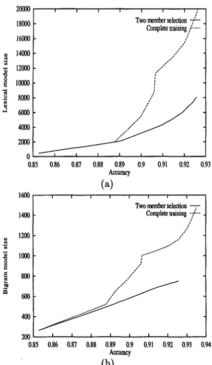
Figure 3: The size of the trained model, measured by t h e number of frequency counts > 0, plotted (y-axis) ver- sus classification accuracy achieved (x-axis). (a) Lexicai

counts (freq(t, w)) (b) Bigram counts (freq(tl--+t2)).

that, to a first approximation, all selection methods considered give similar results. Thus, it seems that a refined choice of the selection m e t h o d is not crucial for achieving large reductions in annotation cost.

This equivalence of the different methods also largely holds with respect to computational effi- ciency. Figure l(b) plots classification accuracy ver-

sus number of words examined, instead of those

selected. We see that while all selective methods

are less efficient in terms of examples examined than complete training, they are comparable to each other. Two member selection seems to have a clear, though small, advantage.

In Figure 2 we investigate further the properties of batch selection. Figure 2(a) shows that accuracy increases with batch size only up to a point, and then starts to decrease. This result is in line with theoretical difficulties with batch selection (Freund et al., 1993) in t h a t batch selection does not account

for the distribution of input examples. Hence, once batch size increases past a point, the input distribu- tion has too little influence on which examples are selected, and hence classification accuracy decreases. Furthermore, as batch size increases, computational efficiency, in terms of the number of examples exam- ined to attain a given accuracy, decreases tremen- dously (Figure 2(5)).

T h e ability of committee-based selection to fo- cus on the more informative parts of the training corpus is analyzed in Figure 3. Here we examined the number of lexical and bigram counts t h a t were stored (i.e, were non-zero) during training, using the two member selection algorithm and complete

training. As the graphs show, the sample selec-

tion m e t h o d achieves the same accuracy as complete training with fewer lexical and bigram counts. This means that m a n y counts in the d a t a a r e less useful for correct tagging, as replacing t h e m with smoothed estimates works just as well. 6 Committee-based se- lection ignores such counts, focusing on parameters which improve the model. This behavior has the practical advantage of reducing the size of the model significantly (by a factor of three here). Also, the average count is lower in a model constructed by selective training than in a fully trained model, sug- gesting t h a t the selection m e t h o d avoids using ex- amples which increase the counts for already known parameters.

7

D i s c u s s i o n

W h y does committee-based sample selection work? Consider the properties of those examples t h a t are selected for training. In general, a selected train- ing example will contribute d a t a to several statistics, which in turn will improve the estimates of several

parameter vMues. An informative example is there-

fore one whose contribution to the statistics leads to a significantly useful improvement of model parame- ter estimates. Model parameters for which acquiring additional statistics is most beneficial can be char- acterized by the following three properties:

1. T h e current estimate of the parameter is uncer- tain due to insufficient statistics in the training set. Additional statistics would bring the esti- mate closer to the true value.

2. Classification of examples is sensitive to changes in the current estimate of the parameter. Oth- erwise, even if the current value of the pa- rameter is very uncertain, acquiring additional statistics will not change the resulting classifi- cations.

3. The parameter affects classification for a large proportion of examples in the input. Parame-

6As noted above, we smooth the MLE estimates by interpolation with a uniform probability distribution (Merialdo, 1994).

[image:6.612.80.293.78.444.2]

ters t h a t affect only few examples have low over- all utility.

T h e committee-based selection algorithms work because they tend to select examples that affect pa-

rameters with the above three properties. Prop-

erty 1 is addressed by randomly drawing the parame- ter values for committee members from the posterior distribution given the current statistics. When the statistics for a parameter are insufficient, the vari- ance of the posterior distribution of the estimates is large, and hence there will be large differences in the values of the parameter chosen for different commit- tee members. Note that property 1 is not addressed when uncertainty in classification is only judged rel- ative to a

single

model 7 (as in, eg, (Lewis and Gale,

1994)).

Property 2 is addressed by selecting examples for

which committee members highly disagree in

clas-

sification

(rather than measuring disagreement in

parameter estimates). Committee-based selection

thus addresses properties 1 and 2 simultaneously: it acquires statistics just when uncertainty in cur- rent parameter estimates entails uncertainty regard-

ing the

appropriate

classification of the example.

Our results show t h a t this effect is achieved even when using only two committee members to sample the space of likely classifications. By

appropriate

classification we mean the classification given by a perfectly-trained model, that is, one with accurate parameter values.

Note that this type of uncertainty regarding the identity of the

appropriate

classification, is differ- ent than uncertainty regarding the

correctness

of the classification itself. For example, sufficient statistics m a y yield an accurate 0.51 probability estimate for a class c in a given example, making it certain that c is the appropriate classification. However, the cer- tainty that c is the

correct

classification is low, since there is a 0.49 chance that c is the wrong class for the example. A single model can be used to estimate only the second type of uncertainty, which does not correlate directly with the utility of additional train- ing.

Finally, property 3 is addressed by independently examining input examples which are drawn from the input distribution. In this way, we implicitly model the distribution of model parameters used for clas- sifying input examples. Such modeling is absent in batch selection, and we hypothesize that this is the reason for its lower effectiveness.

8 C o n c l u s i o n s

Annotating large textual corpora for training natu- ral language models is a costly process. We propose reducing this cost significantly using committee-

rThe use of a single model is also criticized in (Cohn, Atlas, and Ladner, 1994).

based sample selection, which reduces redundant an- notation of examples that contribute little new in- formation. The m e t h o d can be applied in a semi- interactive process, in which the system selects sev- eral new examples for annotation at a time and up- dates its statistics after receiving their labels from

the user. The implicit modeling of uncertainty

makes the selection system generally applicable and quite simple to implement.

Our experimental study of variants of the selec- tion m e t h o d suggests several practical conclusions. First, it was found that the simplest version of the committee-based method, using a two-member com- mittee, yields reduction in annotation cost compa- rable to that of the multi-member committee. The two-member version is simpler to implement, has no parameters to tune and is computationally more ef- ficient. Second, we generalized the selection scheme giving several alternatives for optimizing the m e t h o d for a specific task. For bigram tagging, comparative evaluation of the different variants of the m e t h o d showed similar large reductions in annotation cost, suggesting the robustness of the committee-based approach. Third, sequential selection, which im- plicitly models the expected utility of an example relative to the example distribution, worked in gen- eral better than batch selection. The latter was found to work well only for small batch sizes, where the m e t h o d mimics sequential selection. Increas- ing batch size (approaching 'pure' batch selection) reduces both accuracy and efficiency. Finally, we studied the effect of sample selection on the size of the trained model, showing a significant reduction in model size.

8.1 F u r t h e r r e s e a r c h

Our results suggest applying committee-based sam- ple selection to other statistical NLP tasks which rely on estimating probabilistic parameters from an

annotated corpus. Statistical methods for these

tasks typically assign a probability estimate, or some other statistical score, to each alternative analysis (a word sense, a category label, a parse tree, etc.), and then select the analysis with the highest score. T h e score is usually computed as a function of the estimates of several 'atomic' parameters, often bino- mials or multinomials, such as:

• In word sense disambiguation (Hearst, 1991; Gale, Church, and Varowsky, 1993):

P ( s l f ),

where s is a specific sense of the ambiguous word in question w, and f is a feature of occurrences of w. C o m m o n features are words in the context of w or morphological attributes of it.

• In prepositional-phrase ( P P ) a t t a c h m e n t (Hin-

dle and Rooth, 1993):

P(alf),

where a is a pos- sible attachment, such as an a t t a c h m e n t to a head verb or noun, and f is a feature, or a com- bination of features, of the attachment. Corn-

mon features are the words involved in the at- tachment, such as the head verb or noun, the preposition, and the head word of the PP.

• In statistical parsing (Black et al., 1993): P(rlh), the probability of applying the rule r at a certain stage of the top down derivation of the parse tree given the history h of the deriva- tion process.

• In text categorization (Lewis and GMe, 1994;

Iwayama and Tokunaga, 1994): P(tlC), where

t is a term in the document to be categorized, and C is a candidate category label.

Applying committee-based selection to supervised training for such tasks can be done analogously to its application in the current paper s. ~rthermore, committee-based selection may be attempted also for training non-probabilistic classifiers, where ex- plicit modeling of information gain is typically im-

possible. In such contexts, committee members

might be generated by randomly varying some of the decisions made in the learning algorithm.

Another important area for future work is in de- veloping sample selection methods which are inde- pendent of the eventual learning method to be ap- plied. This would be of considerable advantage in developing selectively annotated corpora for general research use. Recent work on heterogeneous uncer- tainty sampling (Lewis and Catlett, 1994) supports this idea, using one type of model for example selec- tion and a different type for classification.

A c k n o w l e d g m e n t s . We thank Yoav Freund and Yishay Mansour for helpful discussions. The first author gratefully acknowledges the support of the Fulbright Foundation.

R e f e r e n c e s

Black, Ezra, Fred Jelinek, John Lafferty, David Magerman, Robert Mercer, and Salim Roukos. 1993. Towards history-based grammars: using richer models for probabilistic parsing. In Proc. of the Annual Meeting of the ACL, pages 31-37.

Church, Kenneth W. 1988. A stochastic parts pro- gram and noun phrase parser for unrestricted text. In Proc. of ACL Conference on Applied Natural Language Processing.

Cohn, David, Les Atlas, and Richard Ladner. 1994. Improving generalization with active learning.

Machine Learning, 15:201-221.

SMeasuring disagreement in full syntactic parsing is complicated. It may be approached by similar methods to those used for parsing evaluation, which measure the disagreement between the parser's output and the cor- rect parse.

Dagan, Ido and Sean Engelson. 1995. Committee- based sampling for training probabilistic classi- tiers. In Proc. Int'l Conference on Machine Learn- ing, July.

Elworthy, David. 1 9 9 4 . Does Baum-Welch re-

estimation improve taggers? In Proc. of A CL

Conference on Applied Natural Language Process- ing, pages 53-58.

Freund, Y., H. S. Seung, E. Shamir, and N. Tishby. 1993. Information, prediction, and query by com-

mittee. In Advances in Neural Information Pro-

cessing, volume 5. Morgan Kaufmann.

Gale, William, Kenneth Church, and David

Yarowsky. 1993. A method for disambiguating

word senses in a large corpus. Computers and the

Humanities, 26:415-439.

Hearst, Marti. 1991. Noun homograph disambigua- tion using local context in large text corpora. In

Proc. of the Annual Conference of the UW Center for the New OED and Text Research, pages 1-22. Hindle, Donald and Mats Rooth. 1993. Structural

ambiguity and lexical relations. Computational

Linguistics, 19(1):103-120.

Iwayama, M. and T. Tokunaga. 1994. A probabilis- tic model for text categorization based on a sin-

gle random variable with multiple values. In Pro-

ceedings of the .4th Conference on Applied Natural Language Processing.

Johnson, Norman L. 1972. Continuous Multivariate

Distributions. John Wiley & Sons, New York. Kupiec, Julian. 1992. Robust part-of-speech tagging

using a hidden makov model. Computer Speech

and Language, 6:225-242.

Lewis, David D. and Jason Catlett. 1994. Heteroge- neous uncertainty sampling for supervised learn- ing. In Proc. lnt'l Conference on Machine Learn- ing.

Lewis, David D. and William A. Gale. 1994. A sequential algorithm for training text classifiers. In Proc. of the ACM SIGIR Conference.

MacKay, David J. C. 1992. Information-based ob-

jective functions for active data selection. Neural

Computation, 4.

Merialdo, Bernard. 1 9 9 4 . Tagging text with a

probabilistic model. Computational Linguistics,

20(2):155-172.

Press, William H., Brian P. Flannery, Saul A.

Teukolsky, and William T. Vetterling. 1988.

Numerical Recipes in C. Cambridge University Press.

Seung, H. S., M. Opper, and H. Sompolinsky. 1992.

Query by committee. In Proc. A CM Workshop on

Computational Learning Theory.