Combining Association Measures for Collocation Extraction
Pavel PecinaandPavel Schlesinger
Institute of Formal and Applied Linguistics Charles University, Prague, Czech Republic
{pecina,schlesinger}@ufal.mff.cuni.cz
Abstract
We introduce the possibility of combining lexical association measures and present empirical results of several methods em-ployed in automatic collocation extrac-tion. First, we present a comprehensive summary overview of association mea-sures and their performance on manu-ally annotated data evaluated by precision--recall graphs and mean average precision. Second, we describe several classification methods for combining association mea-sures, followed by their evaluation and comparison with individual measures. Fi-nally, we propose a feature selection algo-rithm significantly reducing the number of combined measures with only a small per-formance degradation.
1 Introduction
Lexical association measures are mathematical formulas determining the strength of association between two or more words based on their occur-rences and cooccuroccur-rences in a text corpus. They have a wide spectrum of applications in the field of natural language processing and computational linguistics such as automatic collocation extrac-tion (Manning and Schütze, 1999), bilingual word alignment (Mihalcea and Pedersen, 2003) or de-pendency parsing. A number of various associa-tion measures were introduced in the last decades. An overview of the most widely used techniques is given e.g. in Manning and Schütze (1999) or Pearce (2002). Several researchers also attempted to compare existing methods and suggest differ-ent evaluation schemes, e.g Kita (1994) and Evert (2001). A comprehensive study of statistical as-pects of word cooccurrences can be found in Evert (2004) or Krenn (2000).
In this paper we present a novel approach to au-tomatic collocation extraction based on combin-ing multiple lexical association measures. We also address the issue of the evaluation of association measures by precision-recall graphs and mean
av-erage precision scores. Finally, we propose a step-wise feature selection algorithm that reduces the number of combined measures needed with re-spect to performance on held-out data.
The term collocation has both linguistic and
lexicographic character. It has various definitions but none of them is widely accepted. We adopt the definition from Choueka (1988) who defines
a collocational expressionas “a syntactic and
se-mantic unit whose exact and unambiguous mean-ing or connotation cannot be derived directly from the meaning or connotation of its components”. This notion of collocation is relatively wide and covers a broad range of lexical phenomena such as idioms, phrasal verbs, light verb compounds, tech-nological expressions, proper names, and stock phrases. Our motivation originates from machine translation: we want to capture all phenomena that may require special treatment in translation.
Experiments presented in this paper were per-formed on Czech data and our attention was re-stricted to two-word (bigram) collocations – pri-marily for the limited scalability of some meth-ods to higher-order n-grams and also for the rea-son that experiments with longer word expressions would require processing of much larger corpus to obtain enough evidence of the observed events.
2 Reference data
The first step in our work was to create a refer-ence data set. Krenn (2000) suggests that col-location extraction methods should be evaluated against a reference set of collocations manually extracted from the full candidate data from a cor-pus. To avoid the experiments to be biased by underlying data preprocessing (part-of-speech tag-ging, lemmatization, and parsing), we extracted the reference data from morphologically and syn-tactically annotated Prague Dependency Treebank 2.0 containing about 1.5 million words annotated on analytical layer (PDT 2.0, 2006). A corpus of this size is certainly not sufficient for real-world applications but we found it adequate for our eval-uation purposes – a larger corpus would have made the manual collocation extraction task infeasible.
Dependency trees from the corpus were broken
down intodependency bigramsconsisting of
lem-masof the head word and its modifier, their
part--of-speech pattern, and dependency type. From 87 980 sentences containing 1 504 847 words, we obtained a total of 635 952 different dependency bigrams types. Only 26 450 of them occur in the data more than five times. The less frequent bi-grams do not meet the requirement of sufficient evidence of observations needed by some meth-ods used in this work (they assume normal dis-tribution of observations and become unreliable when dealing with rare events) and were not
in-cluded in the evaluation. We, however, must
agree with Moore (2004) arguing that these cases comprise majority of all the data (the Zipfian phenomenon) and thus should not be excluded from real-world applications. Finally, we filtered out all bigrams having such part-of-speech pat-terns that never form a collocation (conjunction– preposition, preposition–pronoun, etc.) and ob-tained a list consisting of 12 232 dependency
bi-grams, further calledcollocation candidates.
2.1 Manual annotation
The list of collocation candidates was manually processed by three trained linguists in parallel and independently with the aim of identifying colloca-tions as defined by Choueka. To simplify and clar-ify the work they were instructed to select those bigrams that can be assigned to these categories:
∗ idiomatic expressions
- studená válka (cold war)
- visí otazník (question mark is hanging∼open question)
∗ technical terms
- pˇredseda vlády (prime minister) - oˇcitý svˇedek (eye witness)
∗ support verb constructions
- mít pravdu (to be right)
- uˇcinit rozhodnutí (make decision)
∗ names of persons, locations, and other entities
- Pražský hrad (Prague Castle) - ˇCervený kˇríž (Red Cross)
∗ stock phrases
- zásadní problém (major problem) - konec roku (end of the year)
The first (expected) observation was that the in-terannotator agreement among all the categories
was rather poor: the Cohen’s κ between
annota-tors ranged from 0.29 to 0.49, which demonstrates that the notion of collocation is very subjective, domain-specific, and somewhat vague. The reason that three annotators were used was to get a more precise and objective idea about what can be con-sidered a collocation by combining outcomes from
multiple annotators. Only those bigrams that all
three annotators independently recognized as col-locations (of any type) were considered true collo-cations. The reference data set contains 2 557 such
bigrams, which is 20.9% of all. κ between these
two categories reanged from 0.52 to 0.58.
The data was split into six stratified samples. Five folds were used for five-fold cross validation and average performance estimation. The remain-ing one fold was put aside and used as held-out data in experiments described in Section 5.
3 Association measures
In the context of collocation extraction, lexical as-sociation measures are formulas determining the degree of association between collocation
com-ponents. They compute an association scorefor
each collocation candidate extracted from a cor-pus. The scores indicate the potential for a can-didate to be a collocation. They can be used for ranking (candidates with high scores at the top),
or forclassification(by setting a threshold and
dis-carding all bigrams below this threshold).
If some words occur together more often than by chance, then this may be evidence that they have a special function that is not simply explained as a result of their combination (Manning and Schütze, 1999). This property is known in
linguis-tics as non-compositionality. We think of a
cor-pus as a randomly generated sequence of words that is viewed as a sequence of word pairs (de-pendency bigrams in our case). Occurrence fre-quencies and marginal frefre-quencies are used in sev-eral association measures that reflect how much the word cooccurrence is accidental. Such mea-sures include: estimation of joint and conditional
bigram probabilities (Table 1, 1–3), mutual
infor-mation and derived measures (4–9), statistical tests
of independence (10–14), likelihood measures (15–
16), and various other heuristic association
mea-sures and coefficients (17–55) originating in
differ-ent research fields.
By determining the entropy of the immediate
context of a word sequence (words immediately preceding or following the bigram), the
associa-tion measures (56–60) rank collocations according
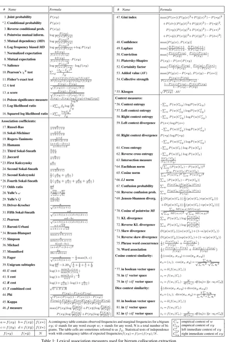
# Name Formula
1.Joint probability P(xy)
?2.Conditional probability P(y|x)
3.Reverse conditional prob. P(x|y)
4.Pointwise mutual inform. logP(xP(xy)∗)P(∗y)
5.Mutual dependency (MD) logP(xP(xy)2∗)P(∗y)
6.Log frequency biasedMD logP(xP(xy)2∗)P(∗y)+logP(xy)
7.Normalized expectation 2f(xy)
f(x∗)+f(∗y)
8.Mutual expectation 2f(xy)
f(x∗)+f(∗y)·P(xy)
?9.Salience log P(xy)2
P(x∗)P(∗y)·logf(xy)
10.Pearson’sχ2test P
i,j (fij−fijˆ )2
ˆ fij
11.Fisher’s exact test N!f(xy)!f(x¯f(x∗)!f(¯x∗)!f(y)!f(¯∗xy)!f(¯y)!f(∗y)!¯x¯y)!
12.ttest √ f(xy)−f(xy)ˆ
f(xy)(1−(f(xy)/N))
13.zscore √ f(xy)−f(xy)ˆ ˆ
f(xy)(1−( ˆf(xy)/N))
14.Poison significance measure f(xy)ˆ −f(xy) log ˆf(xy)+logf(xy)! logN
15.Log likelihood ratio −2Pi,jfijlogfijfijˆ
16.Squared log likelihood ratio −2Pi,jlogfij
2
ˆ fij
Association coefficients:
17.Russel-Rao a a+b+c+d
18.Sokal-Michiner a+d a+b+c+d
19.Rogers-Tanimoto a+d a+2b+2c+d
20.Hamann (a+d)a+b+c+d−(b+c)
21.Third Sokal-Sneath b+c a+d
22.Jaccard a
a+b+c ?23.First Kulczynsky a
b+c
24.Second Sokal-Sneath a a+2(b+c)
25.Second Kulczynski 1
2(a+ba +a+ca ) ?26.Fourth Sokal-Sneath 1
4(a+ba +a+ca +d+bd +d+cd ) ?27.Odds ratio ad
bc
28.Yulle’sω √√ad−√bc
ad+√bc
29.Yulle’sQ ad−bc ad+bc
30.Driver-Kroeber √ a (a+b)(a+c)
31.Fifth Sokal-Sneath √ ad
(a+b)(a+c)(d+b)(d+c)
32.Pearson √ ad−bc
(a+b)(a+c)(d+b)(d+c)
33.Baroni-Urbani a+√ad
a+b+c+√ad
?34.Braun-Blanquet a max(a+b,a+c)
?35.Simpson a
min(a+b,a+c)
36.Michael (a+d)2+(b+c)24(ad−bc)
37.Mountford 2a 2bc+ab+ac
38.Fager √ a
(a+b)(a+c)−
1 2max(b, c)
39.Unigram subtuples logadbc−3.29
q 1
a+1b+1c+1d
40.Ucost log(1+max(b,c)+amin(b,c)+a)
41.Scost log(1+min(b,c)a+1 )−12
42.Rcost log(1+a+ba )·log(1+a+ca )
43.Tcombined cost √U×S×R
44.Phi √ P(xy)−P(x∗)P(∗y)
P(x∗)P(∗y)(1−P(x∗))(1−P(∗y))
45.Kappa P(xy)+P(¯1−P(xx¯y)∗−)P(P(x∗y)∗−)P(P(¯∗y)x∗−)P(P(¯∗xy)¯∗)P(∗y)¯
46.Jmeasure max[P(xy)logP(yP(∗|y)x)+P(xy¯)logP( ¯P(y∗|y)¯x),
P(xy)logP(xP(x|∗y))+P(¯xy)logP(¯P(¯xx|∗y))]
# Name Formula
47.Gini index max[P(x∗)(P(y|x)2+P(¯y|x)2)−P(∗y)2
+P( ¯x∗)(P(y|x¯)2+P(¯y|x¯)2)−P(∗y¯)2,
P(∗y)(P(x|y)2+P(¯x|y)2)−P(x∗)2
+P(∗y¯)(P(x|y¯)2+P(¯x|y¯)2)−P(¯x∗)2]
48.Confidence max[P(y|x), P(x|y)]
49.Laplace max[N PN P(xy)+1(x∗)+2,N P(xy)+1N P(∗y)+2]
50.Conviction max[P(xP(x¯∗)P(y)∗y),P(¯xP(¯∗)P(xy)∗y)]
51.Piatersky-Shapiro P(xy)−P(x∗)P(∗y)
52.Certainity factor max[P(y1|−x)P(−∗P(y)∗y),P(x1|−y)P(x−P(x∗)∗)]
53.Added value (AV) max[P(y|x)−P(∗y), P(x|y)−P(x∗)]
54.Collective strength P(x∗)P(y)+P(¯P(xy)+P(¯xx¯∗y))P(∗y)·
1−P(x∗)P(∗y)−P(¯x∗)P(∗y)
1−P(xy)−P(¯x¯y)
?55.Klosgen pP(xy)·AV
Context measures:
?56.Context entropy −P
wP(w|Cxy) logP(w|Cxy) ?57.Left context entropy −P
wP(w|Cxyl ) logP(w|Cxyl )
58.Right context entropy −PwP(w|Cr
xy) logP(w|Cxyr )
59.Left context divergence P(x∗) logP(x∗)
−PwP(w|Cl
xy) logP(w|Cxyl )
60.Right context divergence P(∗y) logP(∗y)
−PwP(w|Cr
xy) logP(w|Cxyr)
61.Cross entropy −PwP(w|Cx) logP(w|Cy)
62.Reverse cross entropy −PwP(w|Cy) logP(w|Cx)
63.Intersection measure |2Cx|Cx|+∩|CyCy||
?64.Euclidean norm qP
w(P(w|Cx)−P(w|Cy))2
65.Cosine norm
P
w P(w|Cx)P(w|Cy)
P
w P(w|Cx)2·Pw P(w|Cy)2
?66.L1norm P
w|P(w|Cx)−P(w|Cy)|
67.Confusion probability PwP(x|Cw)P(yP(x∗|Cw)P(w)) ?68.Reverse confusion prob. P
wP(y|Cw)P(xP(∗y)|Cw)P(w)
?69.Jensen-Shannon diverg. 1
2[D(p(w|Cx)||12(p(w|Cx)+p(w|Cy)))
+D(p(w|Cy)||12(p(w|Cx)+p(w|Cy)))] ?70.Cosine of pointwiseMI √P Pw MI(w,x)M I(w,y)
w MI(w,x)2·
√P
w MI(w,y)2
71.KL divergence PwP(w|Cx) logP(wP(w||Cx)Cy)
72.Reverse KL divergence PwP(w|Cy) logP(wP(w||Cy)Cx) ?73.Skew divergence D(p(w|C
x)||α(w|Cy)+(1−α)p(w|Cx))
74.Reverse skew divergence D(p(w|Cy)||αp(w|Cx)+(1−α)p(w|Cy))
75.Phrase word coocurrence 1 2(
f(x|Cxy)
f(xy) +
f(y|Cxy)
f(xy) )
76.Word association 1 2(
f(x|Cy)−f(xy)
f(xy) +
f(y|Cx)−f(xy)
f(xy) )
Cosine context similarity: 1
2(cos(cx,cxy)+cos(cy,cxy))
cz= (zi); cos(cx,cy) =
P
xiyi
√P
xi2·√Pyi2
?77.in boolean vector space z
i=δ(f(wi|Cz))
78.intfvector space zi=f(wi|Cz)
79.intf·idfvector space zi=f(wi|Cz)·df(Nwi);df(wi)=|{x:wi²Cx}|
Dice context similarity: 1
2(dice(cx,cxy)+dice(cy,cxy))
cz= (zi); dice(cx,cy) = 2
P
xiyi
P
xi2+Pyi2
80.in boolean vector space zi=δ(f(wi|Cz))
81.intfvector space zi=f(wi|Cz)
82.intf·idfvector space zi=f(wi|Cz)·df(Nwi);df(wi)=|{x:wi²Cx}|
a=f(xy) b=f(xy¯) f(x∗)
c=f(¯xy) d=f(¯xy¯) f(¯x∗)
f(∗y) f(∗y¯) N
A contingency table contains observed frequencies and marginal frequencies for a bigram
xy;w¯stands for any word exceptw;∗stands for any word; N is a total number of bi-grams. The table cells are sometimes referred to asfij. Statistical tests of independence
work with contingency tables of expected frequenciesfˆ(xy) =f(x∗)f(∗y)/N.
Cw empirical context ofw
Cxy empirical context ofxy
Cl
xy left immediate context ofxy
Cr
[image:3.595.76.535.52.749.2]xy right immediate context ofxy Table 1: Lexical association measures used for bigram collocation extraction.
Recall
Precision
0.0 0.2 0.4 0.6 0.8 1.0
0.2
0.4
0.6
0.8
1.0
[image:4.595.308.522.62.201.2]Unaveraged precision curve Averaged precison curve
Figure 1: Vertical averaging of precision-recall curves. Thin curves represent individual non-averaged curves obtained by Pointwise mutual information (4) on five data folds. a specified context window), the association mea-sures rank collocations according to the assump-tion that semantically non-composiassump-tional expres-sions typically occur as (semantic) units in differ-ent contexts than their compondiffer-ents (Zhai, 1997).
Measures (61–74) have information theory
back-ground and measures (75–82) are adopted from the
field of information retrieval.
3.1 Evaluation
Collocation extraction can be viewed as classifi-cation into two categories. By setting a threshold, any association measure becomes a binary clas-sifier: bigrams with higher association scores fall into one class (collocations), the rest into the other
class (non-collocations). Performance of such
classifiers can be measured for example by
accu-racy– fraction of correct predictions. However,
the proportion of the two classes in our case is far from equal and we want to distinguish classifier performance between them. In this case, several
authors, e.g. Evert (2001), suggest usingprecision
– fraction of positive predictions correct and
re-call– fraction of positives correctly predicted. The
higher the scores the better the classification is.
3.2 Precision-recall curves
Since choosing a classification threshold depends primarily on the intended application and there is no principled way of finding it (Inkpen and Hirst, 2002), we can measure performance of associa-tion measures by precision–recall scores within the entire interval of possible threshold values. In this manner, individual association measures can be thoroughly compared by their two-dimensional precision-recall curves visualizing the quality of ranking without committing to a classification threshold. The closer the curve stays to the top and right, the better the ranking procedure is.
Recall
Average precision
0.0 0.2 0.4 0.6 0.8 1.0
0.2
0.4
0.6
0.8
1.0
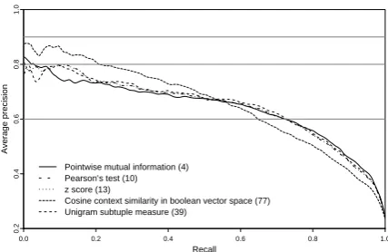
Pointwise mutual information (4) Pearson’s test (10) z score (13)
Cosine context similarity in boolean vector space (77) Unigram subtuple measure (39)
Figure 2: Crossvalidated and averaged precision-recall
curves of selected association measures (numbers in brack-ets refer to Table 1).
Precision-recall curves are very sensitive to data (see Figure 1). In order to obtain a good
esti-mate of their shapescross validationand
averag-ingare necessary: all cross-validation folds with
scores for each instance are combined and a single curve is drawn. Averaging can be done in three
ways:vertical– fixing recall, averaging precision,
horizontal– fixing precision, averaging recall, and combined– fixing threshold, averaging both preci-sion and recall (Fawcett, 2003). Vertical averag-ing, as illustrated in Figure 1, worked reasonably well in our case and was used in all experiments.
3.3 Mean average precision
Visual comparison of precision-recall curves is a powerfull evaluation tool in many research fields (e.g. information retrieval). However, it has a seri-ous weakness. One can easily compare two curves that never cross one another. The curve that pre-dominates another one within the entire interval of recall seems obviously better. When this is not the case, the judgment is not so obvious. Also significance tests on the curves are problematic. Only well-defined one-dimensional quality mea-sures can rank evaluated methods by their per-formance. We adopt such a measure from in-formation retrieval (Hull, 1993). For each
cross--validation data fold we defineaverage precision
(AP) as the expected value of precision for all
pos-sible values of recall (assuming uniform
distribu-tion) andmean average precision(MAP) as a mean
of this measure computed for each data fold. Sig-nificance testing in this case can be realized by paired t-testor by more appropriate nonparametric paired Wilcoxon test.
Due to the unreliable precision scores for low recall and their fast changes for high recall,
esti-mation ofAPshould be limited only to some
[image:4.595.76.289.62.200.2]Mean average precision
0.2
0.3
0.4
0.5
0.6
0.7
773980 3832 3130 13105 4237 427 282963 1622 242345 733 2021 191843 346 54976 503 4882 84459 6673 716126 2515 1114 747268 7053 645249 3565 4169 554047 7581 564612 260 5136 787958 6257 11767 77 38 30 5 4 29 22 45 20 18 6 76 48 44 73 26 11 72 53 49 41 40 81 12 51 79 57 67 67
57 79 51 12 81 40 41 49 53 72 11 26 73 44 48 76 6 18 20 45 22 29 4 5 30 38 77
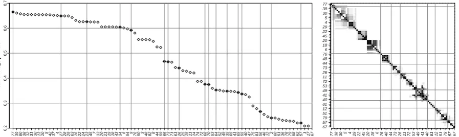
Figure 3: a) Mean average precision of all association measures in descending order. Methods are referred by numbers from Table 1. The solid points correspond to measures selected by the model reduction algorithm from Section 5. b) Visu-alization of p-values from the significance tests of difference between each method pair (order is the same for both graphs). The
darker points correspond to p-values greater thanα= 0.1and indicate methods with statistically indistinguishable performance
(measured by paired Wilcoxon test on values of average precision obtained from five independent data folds).
3.4 Experiments and results
In the initial experiments, we implemented all 82 association measures from Table 1, processed all morphologically and syntactically annotated
sen-tences from PDT 2.0, and computed scores of all
the association measures for each dependency bi-gram in the reference data. For each associa-tion measure and each of the five evaluaassocia-tion data folds, we computed precision-recall scores and drew an averaged precision-recall curve. Curves of some well-performing methods are depicted in Figure 2. Next, for each association measure and each data fold, we estimated scores of average
pre-cision on narrower recall interval h0.1,0.9i,
com-puted mean average precision, ranked the
asso-ciation measures according to MAP in
descend-ing order, and result depicted in Figure 3 a). Fi-nally, we applied a paired Wilcoxon test, detected measures with statistically indistinguishable per-formance, and visualized this information in Fig-ure 3 b).
A baseline system ranking bigrams randomly operates with average precision of 20.9%. The best performing method for collocation
extrac-tion measured by mean average precision is
co-sine context similarity in boolean vector space(77)
(MAP 66.49%) followed by other 16
associa-tion measures with nearly identical performance (Figure 3 a). They include some popular meth-ods well-known to perform reliably in this task,
such as pointwise mutual information(4),
Pear-son’s χ2test(10), zscore(13), odds ratio(27), or
squared log likelihood ratio(16).
The interesting point to note is that, in terms
of MAP, context similarity measures, e.g. (77),
slightly outperform measures based on simple
oc-curence frequencies, e.g. (39). In a more thorough
comparison by percision-recall curves, we observe that the former very significantly predominates the latter in the first half of the recall interval and vice versa in the second half (Figure 2). This is a case
where theMAPis not a sufficient metric for
com-parison of association measure performance. It is also worth pointing out that even if two methods have the same precision-recall curves the actual bi-gram rank order can be very different. Existence
of suchnon-correlated(in terms of ranking)
mea-sures will be essential in the following sections.
4 Combining association measures
Each collocation candidatexican be described by
thefeature vector xi= (xi
1, . . . , xi82)T consisting
of 82 association scores from Table 1 and assigned
a label yi ∈ {0,1} which indicates whether the
bigram is considered to be a collocation (y= 1)
or not (y= 0). We look for a ranker function
f(x)→Rthat determines the strength of lexical
association between components of bigramxand
hence has the character of an association measure. This allows us to compare it with other association measures by the same means of precision-recall curves and mean average precision. Further, we present several classification methods and demon-strate how they can be employed for ranking, i.e. what function can be used as a ranker. For refer-ences see Venables and Ripley (2002).
4.1 Linear logistic regression
An additive model for binary response is
repre-sented by a generalized linear model (GLM) in
a form of logistic regression:
[image:5.595.77.526.65.199.2]method AP MAP R=20 R=50 R=80 R=h0.1,0.9i +
NNet (5 units) 89.56 82.74 70.11 80.81 21.53 NNet (3 units) 89.41 81.99 69.64 79.71 19.88 NNet (2 units) 86.92 81.68 68.33 78.77 18.47
SVM (linear) 85.72 79.49 63.86 75.66 13.79
LDA 84.72 77.18 62.90 75.11 12.96
SVM (quadratic) 84.29 79.54 64.24 74.53 12.09 NNet (1 unit) 77.98 76.83 66.75 73.25 10.17
GLM 82.45 76.26 58.61 71.88 8.11
Cosine similarity (77) 80.94 68.90 50.54 66.49 0.00 Unigram subtuples (39) 74.55 67.49 55.16 65.74
-Table 2: Performance of methods combining all association
measures: average precision (AP) for fixed recall values and
mean average precision (MAP) on the narrower recall interval
with relative improvement in the last column (values in %).
where logit(π) = log(π/(1−π))is a canonical link
function for odds-ratio and π ∈ (0,1) is a
con-ditional probability for positive response given
a vector x. The estimation of β0 and β is done
by maximum likelihood method which is solved
by the iteratively reweighted least squares
algo-rithm. The ranker function in this case is defined
as the predicted value bπ, or equivalently (due to
the monotonicity of logit link function) as the
lin-ear combinationβb0+βbTx.
4.2 Linear discriminant analysis
The basic idea of Fisher’s linear discriminant
anal-ysis (LDA) is to find a one-dimensional projection
defined by a vectorcso that for the projected
com-binationcTxthe ratio of thebetweenvariance B
to thewithinvarianceW is maximized:
max c
cTBc
cTWc
After projection,cTxcan be directly used as ranker.
4.3 Support vector machines
For technical reason, let us now change the labels
yi∈ {-1,+1}. The goal in support vector machines
(SVM) is to estimate a functionf(x) =β0+βTxand
find a classifier y(x) =sign¡f(x)¢which can be
solved through the following convex optimization:
min β0,β
n X
i=1 £
1−yi(β0+βTxi)¤++λ 2||β||
2
with λ as a regularization parameter. Thehinge
loss function L(y,f(x)) = [1−yf(x)]+ is active
only for positive values (i.e. bad predictions) and therefore is very suitable for ranking models with
b
β0+βbTx as a ranker function. Setting the
regu-larization parameter λ is crucial for both the
es-timatorsβb0,βb and further classification (or
rank-ing). As an alternative to a often inappropriate grid
Recall
Average precision
0.0 0.2 0.4 0.6 0.8 1.0
0.2
0.4
0.6
0.8
1.0
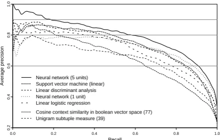
Neural network (5 units) Support vector machine (linear) Linear discriminant analysis Neural network (1 unit) Linear logistic regression
[image:6.595.309.524.63.200.2]Cosine context similarity in boolean vector space (77) Unigram subtuple measure (39)
Figure 4: Precision-recall curves of selected methods com-bining all association measures compared with curves of two best measures employed individually on the same data sets.
search, Hastie (2004) proposed an effective
algo-rithm which fits the entireSVMregularization path
[β0(λ),β(λ)]and gave us the option to choose the
optimal value ofλ. As an objective function we
used total amount of loss on training data.
4.4 Neural networks
Assuming the most common model of neural
net-works (NNet) with one hidden layer, the aim is to
find inner weightswjhand outer weightswhifor
yi=φ0 ¡
α0+ X
whiφh(αh+Xwjhxj) ¢
wherehranges over units in the hidden layer.
Ac-tivation functions φh and function φ0 are fixed.
Typically, φh is taken to be the logistic function
φh(z) = exp(z)/(1 + exp(z)) and φ0 to be the
indicator function φ0(z) =I(z > ∆) with ∆as
a classification threshold. For ranking we simply setφ0(z) =z. Parameters of neural networks are
estimated by thebackpropagation algorithm. The
loss function can be based either onleast squares
or maximum likehood. To avoid problems with
convergence of the algorithm we used the former one. The tuning parameter of a classifier is then the number of units in the hidden layer.
4.5 Experiments and results
To avoid incommensurability of association mea-sures in our experiments, we used a common
pre-processing technique for multivariate
[image:6.595.73.292.65.190.2]on the recall interval h0.1,0.9i. In each cross--validation step, four folds were used for training and one fold for testing.
All methods performed very well in compari-son with individual measures. The best result was achieved by a neural network with five units in the
hidden layer with 80.81% MAP, which is 21.53%
relative improvement compared to the best indi-vidual associaton measure. More complex mod-els, such as neural networks with more than five units in the hidden layer and support vector ma-chines with higher order polynomial kernels, were highly overfitted on the training data folds and bet-ter results were achieved by simpler models. De-tailed results of all experiment are given in Ta-ble 2 and precision-recall curves of selected meth-ods depicted in Figure 4.
5 Model reduction
Combining association measures by any of the presented methods is reasonable and helps in the collocation extraction task. However, the combi-nation models are too complex in number of pre-dictors used. Some association measures are very similar (analytically or empirically) and as predic-tors perhaps even redundant. Such measures have no use in the models, make their training harder,
and should be excluded. Principal component
analysisapplied to the evaluation data showed that 95% of its total variance is explained by only 17 principal components and 99.9% is explained by 42 of them. This gives us the idea that we should be able to significantly reduce the number of vari-ables in our models with no (or relativelly small) degradation in their performance.
5.1 The algorithm
A straightforward, but in our case hardly feasible, approach is an exhaustive search through the space of all possible subsets of all association measures.
Another option is a heuristic step-wisealgorithm
iteratively removing one variable at a time until some stopping criterion is met. Such algorithms are not very robust, they are sensitive to data and generally not very recommended. However, we tried to avoid these problems by initializing our step-wise algorithm by clustering similar variables and choosing one predictor from each cluster as a representative of variables with the same contri-bution to the model. Thus we remove the highly corelated predictors and continue with the step--wise procedure.
Recall
Average precision
0.0 0.2 0.4 0.6 0.8 1.0
0.2
0.4
0.6
0.8
1.0
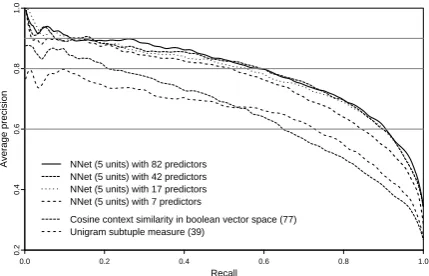
NNet (5 units) with 82 predictors NNet (5 units) with 42 predictors NNet (5 units) with 17 predictors NNet (5 units) with 7 predictors
[image:7.595.309.524.63.201.2]Cosine context similarity in boolean vector space (77) Unigram subtuple measure (39)
Figure 5: Precision-recall curves of four NNet models from the model reduction process with different number of predic-tors compared with curves of two best individual methods.
The algorithm starts with the hierarchical clus-tering of variables in order to group those with a similar contribution to the model, measured by
the absolute value ofPearson’s correlation
coeffi-cient. After 82−diterations, variables are grouped
into dnon-empty clusters and one representative
from each cluster is selected as a predictor into the initial model. This selection is based on individual predictor performance on held-out data.
Then, the algorithm continues withdpredictors
in the initial model and in each iteration removes a predictor causing minimal degradation of
perfor-mance measured by MAP on held-out data. The
algorithm stops when the difference becomes sig-nificant – either statistically (by paired Wilcoxon test) or practically (set by a human).
5.2 Experiments and results
We performed the model reduction experiment on the neural network with five units in the hidden layer (the best performing combination method). The similarity matrix for hierarchical clustering was computed on the held-out data and
parame-terd(number of initial predictors) was
experimen-tally set to 60. In each iteration of the algorithm, we used four data folds (out of the five used in pre-vious experiments) for fitting the models and the held-out fold to measure the performance of these models and to select the variable to be removed. The new model was cross-validated on the same five data-folds as in the previous experiments.
6 Conclusions and discussion
We created and manually annotated a reference data set consisting of 12 232 Czech dependency bigrams. 20.9% of them were agreed to be a col-location by three annotators. We implemented 82 association measures, employed them for collo-cation extraction and evaluated them against the reference data set by averaged precision-recall curves and mean average precision in five-fold cross validation. The best result was achieved by
a method measuring cosine context similarity in
boolean vector spacewith mean average precision of 66.49%.
We exploit the fact that different subgroups of collocations have different sensitivity to certain association measures and showed that combining these measures aids in collocation extraction. All investigated methods significantly outperformed individual association measures. The best results were achieved by a simple neural network with five units in the hidden layer. Its mean average precision was 80.81% which is 21.53% relative improvement with respect to the best individual measure. Using more complex neural networks or a quadratic separator in support vector machines led to overtraining and did not improve the perfor-mace on test data.
We proposed a stepwise feature selection algo-rithm reducing the number of predictors in com-bination models and tested it with the neural net-work. We were able to reduce the number of its variables from 82 to 17 without significant degra-dation of its performance.
No attempt in our work has been made to select the “best universal method” for combining associ-ation measures nor to elicit the “best associassoci-ation measures” for collocation extraction. These tasks depend heavily on data, language, and notion of collocation itself. We demonstrated that combin-ing association measures is meancombin-ingful and im-proves precission and recall of the extraction pro-cedure and full performance improvement can be achieved by a relatively small number of measures combined.
Preliminary results of our research were already published in Pecina (2005). In the current work, we used a new version of the Prague Dependecy Treebank (PDT 2.0, 2006) and the reference data was improved by additional manual anotation by two linguists.
Acknowledgments
This work has been supported by the Ministry of Education of the Czech Republic, projects MSM 0021620838 and LC 536. We would like to thank our advisor Jan Hajiˇc, our colleagues, and anony-mous reviewers for their valuable comments.
References
Y. Choueka. 1988. Looking for needles in a haystack or lo-cating interesting collocational expressions in large textual
databases. InProceedings of the RIAO.
S. Evert and B. Krenn. 2001. Methods for the qualitative
evaluation of lexical association measures. InProceedings
of the 39th Annual Meeting of the ACL, Toulouse, France.
S. Evert. 2004. The Statistics of Word Cooccurrences: Word
Pairs and Collocations. Ph.D. thesis, Univ. of Stuttgart. T. Fawcett. 2003. ROC graphs: Notes and practical
con-siderations for data mining researchers. Technical report, HPL-2003-4. HP Laboratories, Palo Alto, CA.
T. Hastie, S. Rosset, R. Tibshirani, and J. Zhu. 2004. The entire regularization path for the support vector machine.
Journal of Machine Learning Research, 5.
D. Hull. 1993. Using statistical testing in the evaluation of
retrieval experiments. InProceedings of the 16th annual
international ACM SIGIR conference on Research and de-velopment in information retrieval, New York, NY. D. Inkpen and G. Hirst. 2002. Acquiring collocations for
lexical choice between near synonyms. InSIGLEX
Work-shop on Unsupervised Lexical Acquisition, 40th meeting of the ACL, Philadelphia.
K. Kita, Y. Kato, T. Omoto, and Y. Yano. 1994. A compar-ative study of automatic extraction of collocations from
corpora: Mutual information vs. cost criteria. Journal of
Natural Language Processing.
B. Krenn. 2000. The Usual Suspects: Data-Oriented Models
for Identification and Representation of Lexical Colloca-tions. Ph.D. thesis, Saarland University.
C. D. Manning and H. Schütze. 1999.Foundations of
Statis-tical Natural Language Processing. The MIT Press, Cam-bridge, Massachusetts.
R. Mihalcea and T. Pedersen. 2003. An evaluation exercise
for word alignment. InProceedings of HLT-NAACL
Work-shop, Building and Using Parallel Texts: Data Driven Ma-chine Translation and Beyond, Edmonton, Alberta. R. C. Moore. 2004. On log-likelihood-ratios and the
signif-icance of rare events. InProceedings of the 2004
Confer-ence on EMNLP, Barcelona, Spain.
D. Pearce. 2002. A comparative evaluation of collocation
ex-traction techniques. InThird International Conference on
language Resources and Evaluation, Las Palmas, Spain. P. Pecina. 2005. An extensive empirical study of
colloca-tion extraccolloca-tion methods. InProceedings of the ACL 2005
Student Research Workshop, Ann Arbor, USA.
S. Shimohata, T. Sugio, and J. Nagata. 1997. Retrieving col-locations by co-occurrences and word order constraints. InProc. of the 35th Meeting of ACL/EACL, Madrid, Spain.
W. N. Venables and B. D. Ripley. 2002. Modern Applied
Statistics with S. 4th ed. Springer Verlag, New York. C. Zhai. 1997. Exploiting context to identify lexical atoms:
A statistical view of linguistic context. In International