Origin of Dynamic Correlations of Words in Written Texts

(1)

ISSN Online: 2327-7203 ISSN Print: 2327-7211

DOI: 10.4236/jdaip.2019.74014 Oct. 15, 2019 228 Journal of Data Analysis and Information Processing

Origin of Dynamic Correlations of Words in

Written Texts

Hiroshi Ogura, Hiromi Amano, Masato Kondo

Department of Information Science, Faculty of Arts and Sciences, Showa University, Fujiyoshida, Japan

Abstract

In a previous study, we introduced dynamical aspects of written texts by re-garding serial sentence number from the first to last sentence of a given text as discretized time. Using this definition of a textual timeline, we defined an autocorrelation function (ACF) for word occurrences and demonstrated its utility both for representing dynamic word correlations and for measuring word importance within the text. In this study, we seek a stochastic process governing occurrences of a given word having strong dynamic correlations. This is valuable because words exhibiting strong dynamic correlations play a central role in developing or organizing textual contexts. While seeking this stochastic process, we find that additive binary Markov chain theory is useful for describing strong dynamic word correlations, in the sense that it can re-produce characteristics of autocovariance functions (an unnormalized ver-sion of ACFs) observed in actual written texts. Using this theory, we propose a model for time-varying probability that describes the probability of word occurrence in each sentence in a text. The proposed model considers hierar-chical document structures such as chapters, sections, subsections, para-graphs, and sentences. Because such a hierarchical structure is common to most documents, our model for occurrence probability of words has a wide range of universality for interpreting dynamic word correlations in actual written texts. The main contributions of this study are, therefore, finding usability of the additive binary Markov chain theory to analyze dynamic correlations in written texts and offering a new model of word occurrence probability in which common hierarchical structure of documents is taken into account.

Keywords

Autocorrelation Function, Autocovariance Function, Word Occurrence, Stochastic Process, Additive Binary Markov Chain

How to cite this paper: Ogura, H., Amano, H. and Kondo, M. (2019) Origin of Dy-namic Correlations of Words in Written Texts. Journal of Data Analysis and Information Processing, 7, 228-249. https://doi.org/10.4236/jdaip.2019.74014

Received: August 26, 2019 Accepted: October 12, 2019 Published: October 15, 2019

(2)

DOI: 10.4236/jdaip.2019.74014 229 Journal of Data Analysis and Information Processing

1. Introduction

Introducing the notion of time to written texts reveals dynamical aspects of word occurrences, allowing us to apply standard dynamical analyses developed and used in the fields of signal processing and time series analysis. In a previous study [1], we used a set of serial sentence numbers assigned from the first to last sentence in a given text as a discretized time. Using this time unit, we success-fully defined an autocorrelation function (ACF) appropriate to words in written texts, then calculated ACFs according to this definition for words frequently ap-pearing in twelve famous books. We found that the resulting ACFs could be classified into two groups: words showing dynamic correlations and those with no correlation type. Words showing dynamic correlations are called Type-I words, and their ACFs are well-described by a modified Kohlrausch-Williams-Watts (KWW) function. Words showing no correlation are called Type-II words, and their ACFs are modeled as a simple stepdown function. We showed that this stepdown function can be theoretically derived from the assumption that the stochastic process governing occurrences of Type-II words is a homogeneous Poisson point process.

Type-I words are known to occur multiple times in a text in a bursty and con-text-specific manner, and such occurrences ensure that the word has a dynamic correlation. Put another way, Type-I words are important for describing an idea or topic, and are therefore expected to be highly correlated with a duration, typ-ically several tens of sentences in which the idea or topic is described. In con-trast, Type-II words are not context-specific and their appearance is governed by chance. Type-I words are therefore more important than Type-II words, in the sense that they play a central role in explaining the author’s ideas or thoughts. The author’s insights and thought process should thus be discernible through modeling of the stochastic process that generates Type-I words. However, de-spite the importance of Type-I words, the stochastic process yielding them could not be clarified in the previous study.

(3)

eas-DOI: 10.4236/jdaip.2019.74014 230 Journal of Data Analysis and Information Processing ily converted to a time-varying probability having the two features described above. We constructed this recursive model by incorporating common hierar-chical document structures (chapters, sections, subsections, paragraphs, and sentences), so it can be applied to a broad range of applications for analyzing written texts. Although long-range correlations in written texts have been mod-eled from various point of views, the methodologies used are completely differ-ent from ours [3] [4].

The remainder of this paper is organized as follows: In Section 2, we define the autocovariance function (ACVF), an unnormalized ACF used throughout this study. In Section 3, we describe the additive binary Markov chain theory, which allows mutual conversion between memory functions and ACVFs. We also present the relation between the time-varying probability of word occurrence and the memory function, which allows us to estimate the time-varying probability of a given word. In Section 4, we present typical examples of time-varying proba-bility for Type-I words and their two distinctive features. In Section 5, we de-scribe how to establish a recursive model for a probability distribution that successfully reproduces the two features of the time-varying probability. Final-ly, in Section 6, we present our conclusions and suggest directions for future re-search.

2. Autocorrelation and Autocovariance Functions

2.1. Definitions of Autocorrelation and Autocovariance Functions

The autocovariance function gives the covariance of a given process with itself at pairs of time points. A standard definition of the ACVF for a weak stationary process

{ }

Xt is

( )

(

t

)(

t

)

,

K τ =E X −µ X+τ−µ  (1)

where E

[ ]

is an expectation operator and µ =E X

[ ]

t is the mean of

{ }

Xt

[5] [6]. The ACF, which measures the similarity between signals Xt as a

func-tion of the time lag

τ

between them, is a normalized autocovariance defined as [5] [6]

( )

_{( )}

. 0

K K

τ

ρ τ = (2)

As Equation (1) and Equation (2) show, these definitions for ACVF and ACF use the deviation of Xt from its mean instead of Xt itself. In our previous

study [1], we used Xt itself to define the ACF so that the limit of the ACF at

infinitely large

τ

gives important information regarding Type-II words, that is, the limit of ACF using Xt itself approaches a constant rate λ of a

corres-ponding homogeneous Poisson point process for a given Type-II word when

(4)

DOI: 10.4236/jdaip.2019.74014 231 Journal of Data Analysis and Information Processing Another difference between the previous and present studies is that we exten-sively use ACVFs instead of ACFs because ACVFs more directly link to additive binary Markov chain theory, as will be shown later.

2.2. Examples of ACVFs for Type-I and Type-II Words

Because we use the set of serial sentence numbers assigned from the first to the last sentence in a considered text as discretized time, and because we intend to analyze word occurrence characteristics in terms of ACVFs, we define the signal

t

X representing word occurrence or non-occurrence as

(

)

(

)

1 when a given word occurs in the th sentence 0 when a given word does not occur in the th sentence

t

t X

t

 = 

[image:4.595.210.539.487.669.2]

 (3)

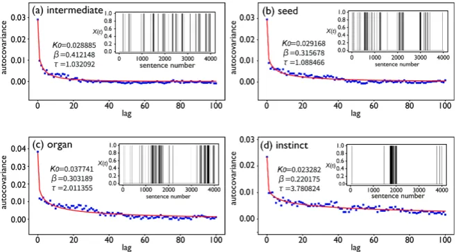
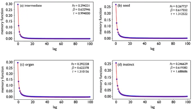
Figure 1 and Figure 2 show examples of Xt and ACVFs calculated from t

X for typical Type-I and Type-II words, respectively, extracted from a set of frequent words in Charles Darwin’s most famous work, On the Origin of Species. These words were chosen as typical Type-I and Type-II words in the previous study, and are also used here for comparison. Here, a “frequent” word is one appearing in at least 50 sentences in the text. Text preprocessing procedures performed before calculating ACVFs are the same as in the previous study.

As Figure 1 shows, ACVFs—namely K

( )

τ _{as defined in Equation (1)—for} Type-I words are monotonically decreasing, indicating that dynamic correla-tions decrease as lag τ increases. They also show an apparent persistence of dy-namic correlations with durations of several tens of sentences. In contrast, Fig-ure 2 clearly shows that ACVFs for Type-II words show no dynamic correlations, suggesting that Type-II words are generated from a memoryless stochastic process. Figure 1 and Figure 2 show that the functional forms and characteristic behaviors of ACVFs are the same as those for the corresponding ACFs reported

Figure 1.Examples of Xt (insets) and ACVFs (blue plots) for typical Type-I words. Red

curves represent the best-fitted KWW functions (see Section 4) of which optimized pa-rameters are shown in the plot areas. Xt and ACVFs for (a) “intermediate”, (b) “seed”, (c)

(5)

[image:5.595.211.534.62.219.2]

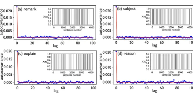
Figure 2.Examples of Xt (insets) and ACVFs (blue plots) for typical Type-II words. Red

lines represent the stepdown functions. Xt and ACVFs for (a) “remark”, (b) “subject”, (c)

“explanation”, and (d) “reason”, from a set of frequently used words in the Darwin text.

in the previous study. Therefore, the model functions used in the previous study to describe the ACFs of Type-I and Type-II words are still appropriate for de-scribing ACVFs for each word type. Specifically, the Kohlrausch-Williams-Watts (KWW) function used to model the ACFs of Type-I words and the stepdown function used to describe the ACFs of Type-II words still provide full descriptive power when applied to modeling ACVFs. Figure 1 and Figure 2 show fitting results from these two model functions as red lines, indicating the validity of us-ing KWW and the stepdown functions to model the two ACVF types. Details of the fitting results using the KWW function for the ACVFs of Type-I words will be described in Section 4.

Our previous study found that, without exception, all frequent words appear-ing in the twelve famous books are well classified into Type-I or Type-II words. This study also showed that the stochastic process governing occurrences of Type-II words is a homogeneous Poisson point process, which is completely memoryless. In the following section, we describe our attempts to determine a stochastic process for generating Type-I words in written text. We also investi-gate a mechanism for providing dynamic correlations to Type-I words.

3. Additive Binary Markov Chain

3.1. Necessity of an Additive Markov Chain

One standard approach to analyzing time series with dynamic correlations is to use a Markov chain model [7] [8] [9]. Because a first-order Markov chain is sim-plest, we first apply one to model Type-I word occurrences and check whether or not the model can reproduce actual ACVFs exhibiting dynamic correlations. Consider a random variable Xt where t denotes a discretized time. If the

proba-bility of moving to the next state at the next time depends only on the present state, that is, if

(

n 1 | 1 1, 2 2, , n n

)

(

n 1 | n n

)

Pr X + =x X =x X =x  X =x =Pr X + =x X =x (4)

(6)

DOI: 10.4236/jdaip.2019.74014 233 Journal of Data Analysis and Information Processing chain in which signal Xt takes only values 0 or 1 as in Equation (3), the

sto-chastic properties of the first-order Markov chain can be completely determined by defining a transition matrix

00 10 01 11 , P P P P P   =  

  (5) where Pij denotes a transition probability from state i to state j. To determine

all values of Pij in the transition matrix from signals

{ }

Xt observed in actual

written texts, we simply used maximum likelihood estimators

0 1 , ij ij i i n P n n =

+ (6) where nij is the number of transitions from state i to state j observed in signals

{ }

Xt . Table 1 shows transition probabilities thus obtained for the typical Type-I

words shown in Figure 1.

After obtaining all values of Pij listed in Table 1, we can simulate

occur-rences of a given word by using a simple Monte Carlo procedure as follows: 1) Arbitrarily set an initial state X0 as 0 or 1.

2) Determine the next state X1, by comparing P00 or P10 with a generated random number p∈

[ ]

0,1 following the standard uniform distribution U

( )

0,1 . If the initial state was X0=0, compare random number p with P00. Otherwise, if X0=1, compare p with P10. For example, consider the case where X1=0. Then if p P< 00 we set the next state as X1=0, while if p P≥ 00 we set

1 1

X = _{. This procedure ensures that}Pr X

(

₁=0 |X₀ =0

)

=P₀₀ and

(

1 1| 0 0

)

01

Pr X = X = =P because from Equation (6), P00+P01=1 always holds. Similarly, given X0=1, if p P< 10 we set X1=0, otherwise we set X1=1 so that Pr X

(

1=0 |X0= =1

)

P10 and Pr X

(

1=1|X0= =1

)

P11.

3) Repeat Step 2 with replacements X1→Xi and X0→Xi−1

(

i=2,3, , n

)

. By repeating this procedure n times, we can obtain simulated signals

1, 2, , n

X X  X , the set of which is a first-order Markov chain having the transi-tion matrix P given by Equatransi-tion (5).

Insets in Figure 3 show examples of simulated signals Xt for typical Type-I

words with transition matrices P, elements of which are listed in Table 1. That figure also shows ACVFs calculated from those simulated signals. Obviously, these ACVFs are completely different from the actual ACVFs shown in Figure 1, in that they do not have long durations over several tens of sentences, although they exhibit dynamic correlations over much shorter durations. This indicates that the first-order Markov chain cannot reproduce actual dynamic correlations of Type-I words.

A direct and intuitive way to discover dynamic correlations with long dura-tions in simulated signals Xt is to consider higher-order Markov chains [7] [8]

[9]. In an mth order Markov chain, the probability of moving to the next state is

(

)

(

1 1 1 11 2 21 2 2

)

| , , ,

| , , , .

n n n

n n m n m n m n m n n

Pr X x X x X x X x

Pr X x X x X x X x

+

+ − + − + − + − +

= = = =

= = = = =



(7)

[image:7.595.209.539.88.369.2]

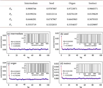
Table 1. Transition probabilities for typical Type-I words estimated by Equation (6).

Intermediate Seed Organ Instinct

P00 0.9800766 0.9787887 0.9723871 0.9860371 P01 0.0199234 0.0212114 0.0276129 0.0139629 P10 0.6446281 0.6747967 0.6645963 0.5670103 P11 0.3553719 0.3252033 0.3354037 0.4329897

Figure 3.Simulated signals Xt (insets) for the typical Type-I words obtained as a

realiza-tion of first-order Markov chains and ACVFs (blue plots) calculated from those Xt. Red

curves represent best-fitted KWW functions, optimized parameters for which are shown in the plot areas. Results are for the words (a) “intermediate”, (b) “seed”, (c) “organ”, and (d) “instinct”.

However, one difficulty is that the number of transition probabilities, each of which is an element of the transition matrix, grows exponentially with the order. In the case of binary Markov chains, we must evaluate ₂m+1_transition proba-bilities to model the mth order Markov chain because we must consider all possi-ble transition patterns in the last m signals. If m=10_{, we must determine 2048}

transition probabilities. This is impossible because we cannot obtain sufficient samples to evaluate these probabilities when the number of signals Xt, which is

equal to the number of sentences in the considered text, is the same order as the number of transition probabilities to be evaluated. For example, The Origin of Species has 3991 sentences, so it is impossible to determine 2048 transition proba-bilities with sufficient statistical reliability from 3991 signals. We must therefore consider another model that is tractable and can generate dynamic correlations with long durations. In the following subsection, we introduce additive binary Markov chains for this purpose.

3.2. Framework of Additive Binary Markov Chain Theory

(8)

DOI: 10.4236/jdaip.2019.74014 235 Journal of Data Analysis and Information Processing show that the theory is successfully applied to model occurrences of Type-I words.

An additive Markov chain of order m has the property

(

| 1 1, 2 2, ,

)

1

(

, , .

)

m

n n n n n n n m n m r n n r

Pr X =x X − =x− X − =x−  X − =x− =

∑

= f x x− r (8)

This means influences of previous states at different times are mutually inde-pendent on next states and thus can be expressed in additive form. In the binary case, where signal Xt is restricted to a value of 0 or 1, the theory tells us that

the conditional probability of Equation (8) can be modified as

(

)

( )

(

)

1 1 2 2

1

1| , , ,

,

n n n n n n m n m

m

n r r

Pr X X x X x X x

X F r x X

− − − − − − − = = = = = = +

∑

−  (9)

where X is the mean of signals

{ }

Xt , and F r

( )

is a memory function

representing the degree of influence of a previous signal occurring r time steps before. Thus, if F r

( )

takes a large value, then the occurrence of a given word

at t n r= − _{positively affects the word occurrence at}t n= _{. Another}

implica-tion of Equaimplica-tion (9) is that by obtaining F r

( )

for a given word, we can calcu-late the probability of signal Xt being 1 by this equation, and we can therefore

generate signals Xt by use of a simple Monte Carlo procedure with that

prob-ability. Because the parameters needed to simulate generation of Xt are F r

( )

,

the number of parameters to be evaluated is equal to the order m of the consi-dered additive Markov chain. Tractability is therefore greatly improved because the number of parameters is only linearly dependent on the order m of a consi-dered Markov chain.

Furthermore, the theory of additive binary Markov chains [10] [11] offers simple simultaneous equations that directly relate ACVFs—K r

( )

given by Eq-uation (1)—to the memory functions F r

( )

appearing in Equation (9) as

( )

(

) ( ) (

)

1 1,2, ,

m

s

K r K r s F s r m

=

∑

− =  (10)

Note that the relations

( )

,

K r =K r− (11)

( )

0

(

1

)

,

K =X −X ₍₁₂₎

always hold by the definition of K r

( )

. By using Equation (11) and Equation (12), we can regard Equation (10) as m simultaneous equations relating ACVFs

( ) ( )

1 , 2 , ,

( )

K K  K m to memory functions F

( ) ( )

1 ,F 2 , , F m

( )

. We can thus calculate ACVFs, K r

( )

, from a theoretically assumed memory function F r

( )

, or we can conversely calculate memory functions F r

( )

for a given word at

1,2, ,

r= _ m_{from its actual ACVFs.}

Before applying additive binary Markov chain theory to analyze dynamic cor-relations for Type-I words, we confirm the validity of the theory as follows. First, we assume the tentative memory function

( )

(

)

(

)

0.1 0.05 1 20

0 20

r r

F r

r

− ≤ <

 = 

≤

(9)

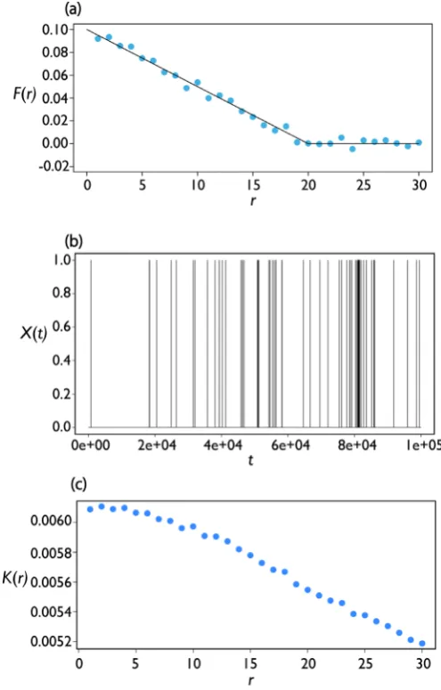
DOI: 10.4236/jdaip.2019.74014 236 Journal of Data Analysis and Information Processing which is shown as the solid line in Figure 4(a). This function is plausible in the sense that memory decreases as lag r increases. We set other conditions as

0.05

X = _and X₀=0_{, tentatively determined to fit actual word occurrences.} We then generate signals Xt according to the conditional probability given by

Equation (9) using a simple Monte Carlo procedure, the algorithm for which is basically the same as that for generating

{ }

Xt using the first-order Markov

chain. The Monte Carlo simulation to generate Xt applies two conditions (C1)

and (C2), as follows:

[image:9.595.248.496.295.683.2]

(C1) Signal Xn=1 if a generated random number p∈

[ ]

0,1 following standard uniform distribution U

( )

0,1 is less than the conditional probability given by Equation (9). Otherwise, Xn =0. To calculate the conditional proba-bility, we substitute F r

( )

as calculated from Equation (13) and the past m signal values into Equation (9). This procedure is repeated until we obtain the desired length of signals

{ }

Xt .

Figure 4.(a) Memory function F(r) given by Equation (13) (solid line) and reproduced

F(r) from ACVFs with Equation (10) (blue plots); (b) Simulated signals Xt generated by a

(10)

DOI: 10.4236/jdaip.2019.74014 237 Journal of Data Analysis and Information Processing (C2) The number of past signals is insufficient for generating the first m−2

signals X X1, 2, , Xm−2 because Equation (9) requires past m signals 1, 2, ,

n n n m

X − X −  X − to calculate the conditional probability of Xn being 1. In

these cases, we use all available past n signals from X0 to Xn−1 to calculate Equation (9) and ignore other terms that require X X−1, −2,.

Obtained Xt and estimated ACVFs from Xt with a condition m=30 are

shown in Figure 4(b) and Figure 4(c), respectively. The functional form of ACVFs (Figure 4(c)) is very similar to the used memory function (the solid line in Figure 4(a)), which is consistent with previously reported results [10] [11]. To confirm the validity of the additive binary Markov chain theory, we calculate values for the memory function F r

( )

from ACVFs in Figure 4(c) by inversely using the simultaneous equations, Equation (10). Figure 4(a) compares the memory function calculated from ACVFs (blue plots) and that of the original Equation (13) (solid line). As that figure shows, the original and calculated

( )

F r from ACVFs satisfactorily agree, ensuring validity of the theory. The fol-lowing section applies additive binary Markov chain theory as a basic framework for investigating characteristics of the stochastic process that generates Type-I words.

4. Memory Functions and Occurrence Probabilities of Type-I

Words

In this section, we apply the theory of additive binary Markov chain to Type-I word occurrences to clarify characteristics of the stochastic process that gene-rates dynamic correlations of Type-I words. Since ACVFs for Type-I words can be calculated from actual signals Xt by use of Equation (1) and these ACVFs

can be used as observed K r

( )

values in Equation (10), it is easy to determine

( )

[image:10.595.210.539.493.680.2]

F r values at each lag r from Equation (10). Figure 5 shows examples of thus

Figure 5.Examples of F(r) (blue plots) for typical Type-I words calculated from ACVFs

(11)

DOI: 10.4236/jdaip.2019.74014 238 Journal of Data Analysis and Information Processing obtained F r

( )

for typical Type-I words. When calculating F r

( )

, we have used K r

( )

represented by best-fitted KWW functions at each lag step instead of the original ACVFs to reduce noise effects. Red lines in that figure represent results fitted to F r

( )

by use of KWW functions, indicating that memory func-tions F r

( )

for Type-I words can also be well described by KWW functions as in the case of fitting ACVFs.

Strictly speaking, because the memory function F r

( )

is defined at r≥1, as seen in Equation (9) and Equation (10), we use a modified form of the KWW function for F r

( )

:

( )

0exp r 1 ,

F r F

β τ  ₋      = _−_ _ _    

  (14)

while when fitting ACVFs we use the standard form of the KWW function, namely,

( )

0exp r .

K r K

β τ       = _−_{ } _    

[image:11.595.209.539.627.725.2]

  (15)

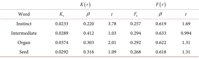
Table 2 summarizes the evaluated fitting parameters of the KWW functions, Equation (14) and Equation (15), obtained through fittings for the typical Type-I words. These optimized parameters are obtained by nonlinear least-squares fit-ting. Fitting parameters for K r

( )

are more scattered than those for F r

( )

, particularly in values of

β

_and

τ

. This means that slight differences in func-tional form for F r

( )

are amplified and become distinct in K r

( )

.

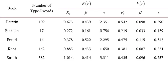
To confirm this observation, we conducted nonlinear least-squares fittings for all Type-I words from five well-known academic books, described in detail in the Appendix. Table 3 summarizes means and standard deviations of the fitting parameters for the Type-I words, and Table 4 lists coefficients of variation (CV), defined as σ µ_{and calculated from the data in}_{Table 3}_._{Table 4}_reconfirms that fitting parameter values are more scattered for K r

( )

than for F r

( )

be-cause CVs of

β

and

τ

for K r

( )

are much larger than those for F r

( )

.

Consistency of the additive binary Markov chain theory for modeling occur-rences of Type-I words can be used to confirm whether the theory can reproduce observed ACVFs. The procedure for confirming consistency is as follows. Note that we use the symbol Xt for actual signals of word occurrence or

nonoccur-rence as observed in actual written text, and Xn designates simulated signals

obtained through simple Monte Carlo procedures.

Table 2. Optimized fitting parameters of Equations (14) (F(r)) and (15) (K(r)) obtained by nonlinear least-squares fitting.

( )

K r F r

( )

Word K0 β τ F0 β τ

Instinct 0.0233 0.220 3.78 0.257 0.619 1.69 Intermediate 0.0289 0.412 1.03 0.294 0.633 0.994

Organ 0.0374 0.303 2.01 0.292 0.622 1.31

(12)

[image:12.595.62.539.105.228.2]

Table 3. Mean µ and standard deviation

σ

for fitting parameters in K r

( )

(Equation (15)) and F r

( )

(Equation (14))

calculated for all Type-I words appearing in the corresponding book and described in the form µ σ± .

Book _{Type-I words}Number of K r

( )

F r

( )

0

K β τ F0 β τ

Darwin 109 0.0278 ± 0.0187 0.262 ± 0.115 0.485 ± 1.14 0.142 ± 0.0769 0.584 ± 0.0574 1.88 ± 0.545 Einstein 17 0.0732 ± 0.0199 0.261 ± 0.0420 0.224 ± 0.169 0.161 ± 0.0353 0.589 ± 0.0195 1.77 ± 0.281 Freud 14 0.0465 ± 0.0176 0.276 ± 0.144 0.658 ± 1.51 0.160 ± 0.0760 0.596 ± 0.0683 1.81 ± 0.564 Kant 142 0.0283 ± 0.0250 0.245 ± 0.106 0.237 ± 0.391 0.140 ± 0.0534 0.580 ± 0.0506 1.97 ± 0.442 Smith 382 0.0141 ± 0.0143 0.256 ± 0.106 0.305 ± 1.01 0.131 ± 0.0570 0.583 ± 0.0561 1.91 ± 0.491

Table 4. CV for the fitting parameters in K r

( )

(Equation (15)) and F r

( )

(Equation (14)) calculated from σ µ values in Table 3.

Book _{Type-I words}Number of K r

( )

F r

( )

0

K β τ F0 β τ

Darwin 109 0.673 0.439 2.351 0.542 0.098 0.290 Einstein 17 0.272 0.161 0.754 0.219 0.033 0.159 Freud 14 0.378 0.522 2.295 0.475 0.115 0.312 Kant 142 0.883 0.433 1.650 0.381 0.087 0.224 Smith 382 1.014 0.414 3.311 0.435 0.096 0.257

1) ACVFs for a Type-I word are calculated using Equation (1) from actual signals Xt observed in the text.

2) Curve fitting to fit Equation (15) to ACVFs obtained in the previous step is performed to obtain optimized values for fitting parameters.

3) K r

( )

is calculated at each lag step r using Equation (15) with the opti-mized fitting parameters. We set the maximum lag step as rmax =100, which, as will be recognized in the following steps, is equivalent to setting the order of the additive binary Markov chain to m=100. This setting is sufficient to cover the longest durations of dynamic correlations for Type-I words [1].

4) K r

( )

obtained in the previous step are substituted into the simultaneous equations, Equation (10), to obtain F r

( )

.

5) F r

( )

is used to calculate the conditional probability, Equation (9), and the calculated conditional probability of Xn being 1 is used to generate

simu-lated signals Xn through simple Monte Carlo procedures. Conditions (C1) and

(C2) described in Subsection 3.2 are still applied in this step. Before starting the Monte Carlo procedures, we set X to the averaged value of actual signals for a given word.

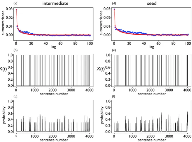
6) From the simulated signals Xn, ACVFs are calculated using Equation (1)

[image:12.595.210.539.279.401.2]

(13)

DOI: 10.4236/jdaip.2019.74014 240 Journal of Data Analysis and Information Processing Figure 6(a) and Figure 6(d) show comparisons between ACVFs calculated from actual signals (blue plots) and those reproduced from simulated signals (red plots) for two typical Type-I words, “intermediate” and “seed”. Both are in good agreement, indicating that dynamic correlations of Type-I words are well modeled by the theory of additive binary Markov chains. Figure 6 also shows simulated signals Xn obtained through the simple Monte Carlo procedures

(Figure 6(b) and Figure 6(e)) and the conditional probabilities of Xn being 1

(Figure 6(c) and Figure 6(f)).

As Equation (9) shows, signals Xt are considered to be consequences of the

time-varying conditional probabilities for word occurrence given by Equation (9) in the framework of additive binary Markov chain theory. In this sense, the un-observed time-varying probabilities given by Equation (9) are more essential than the observed signals Xt. The time-varying probabilities shown in Figure

6(c) and Figure 6(f) seem plausible in the sense that the probabilities take high-er values in time inthigh-ervals with highhigh-er word occurrence rates.

[image:13.595.211.539.414.656.2]

A closer look at Figure 6(c) and Figure 6(f) reveals two further characteristics of the time-varying probability: that the probability value does not continuously change, but instead seems to be discretized to form several levels in an approx-imate sense, and that same-level probabilities seem to aggregate within a certain period of time. That is, the sentence numbers at which the occurrence probabil-ity takes approximately the same values among several discretized values seem to be aggregated along the time (sentence number) axis.

Figure 6.(a) and (d) ACVFs calculated from actual signals Xt observed in the text (blue

plots) and those reproduced from simulated signals Xn (red plots); (b) and (e) Simulated

signals Xn generated using the simple Monte Carlo procedures; (c) and (f) Conditional

probabilities of Xn being 1 calculated using Equation (9). The left and right columns show

(14)

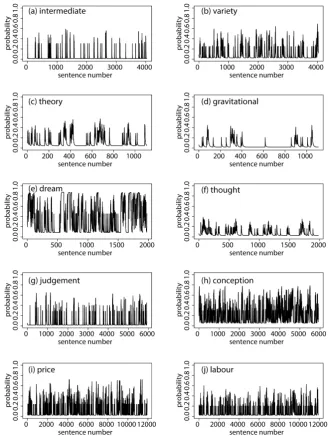
DOI: 10.4236/jdaip.2019.74014 241 Journal of Data Analysis and Information Processing We further calculated the time-varying probabilities of Xn being 1 for

[image:14.595.207.538.184.621.2]

typi-cal Type-I words selected from five academic books. Specifitypi-cally, we chose the two words having the largest and second largest ΔBIC in each book because ΔBIC is a measure of dynamic correlation and thus indicates the importance of a given word [1]. Figure 7 shows the results for the words selected in this way. As that figure shows, the two features described above are common among all cases, indicating that the two features are substantial for all Type-I words having

Figure 7. Conditional probabilities of Xn being 1 calculated using Equation (9). The

(15)

DOI: 10.4236/jdaip.2019.74014 242 Journal of Data Analysis and Information Processing strong dynamic correlations, although the second feature (aggregation along the horizontal axis) is not easy to see in Figures 7(g)-(j) due to compression of the horizontal axes.

The two features described above cannot be directly explained from Equation (9), so another viewpoint beyond the scope of additive binary Markov chain theory is needed to explain them. In the following section, we propose a recur-sive probability distribution model in which hierarchical structures of docu-ments are considered to explain these features.

5. Hierarchical Model of Probability Distribution for Word

Occurrences

Almost all documents have a hierarchical structure consisting of chapters, sec-tions, subsecsec-tions, paragraphs, and sentences. This section describes the con-struction of a probability distribution model that reflects such hierarchical structures. The constructed model is expected to reproduce the two features of the time-varying probability of word occurrence described in the previous sec-tion. However, because our aim is to capture dynamic correlations of Type-I words with a simple model and we do not intend to build a complex or sophisti-cated model, some details of the proposed model will be tentatively determined. We believe, however, that the hierarchical structures of documents induce dy-namic correlations of Type-I words, and that our model essentially captures the origin of these correlations.

Our model is based on a recursive probability redistribution that constructs a hierarchical probability distribution. After obtaining the hierarchical probability distribution, we convert it to the time-varying probability of word occurrence. The probability redistribution and conversion are performed in the following manner.

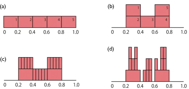
1) As a starting point, we consider the standard uniform distribution U

( )

0,1 illustrated in Figure 8(a), in which the density function is fixed to 1 in the unit interval [0, 1] and 0 otherwise. 0 and 1 on the horizontal axis correspond to the positions of the first and the last sentences in the text, so the unit interval [0, 1] corresponds to the entire text. No structures are introduced in the distribution at this point, so the occurrence probability of a given word is exactly the same for all sentences in the text.

2) The unit interval [0, 1] is divided into 5 subintervals of the same length, indexed as 1, 2, 3, 4, 5 (Figure 8(a)). These subintervals correspond to five chapters in the text. We then select two indices, a1 and a2, taken from a discrete uniform distribution with possible values

{

1,2,3,4,5

}

. Here, we select two other indices, b1 and b2, differing from a1 and a2 by sampling without replace-ment.

3) The rectangles representing probabilities at subintervals with indices a1 and a2 are removed and stacked on rectangles having indices b1 and b2. In

(16)

[image:16.595.216.535.67.218.2]

Figure 8.The procedure for probability redistribution considering hierarchical structures

in the actual written text.

zero, indicating that chapters 1 and 5 become irrelevant to descriptions using the considered word, while chapters 2, 3, and 4 are considered relevant.

4) Division into five subintervals, choosing indices a1, a2, b1, and b2 and the stacking of probabilities are repeated for each portion of the top layer in the probability distribution as in Figure 8(c) and Figure 8(d). This procedure is recursively repeated to form a desired hierarchical structure for the probability distribution. For example, if we repeat this procedure twice, we obtain the prob-ability distribution in Figure 8(d) with four different density function values (zero and three positive values 1, 2 and 3). Similarly, by repeating this three times, we obtain a probability distribution with five function values.

5) After obtaining a desired hierarchical probability distribution, that is, after repeating the probability redistribution a predefined number of times, we dis-cretize the horizontal axis and convert it into sentence numbers. For example, if we repeat the previous step three times, that is, if we set the number of repeti-tions as r=3_{, then the unit interval [0, 1] is divided into} ₅3₌₁₂₅_{subintervals,} considered to be 125 sentences with serial sentence number from 1 to 125. In this case, because the text length of 125 sentences is too short to calculate ACVFs with statistical reliability, we concatenate 10 different obtained hierarchical probability distributions, each having 125 sentences to form a text with 1250 sentences. Concatenation of 10 hierarchical probability distributions is applied to the cases of r=2,3,4_{and concatenation of 5 hierarchical probability} dis-tributions is used for r=5_.

(17)

DOI: 10.4236/jdaip.2019.74014 244 Journal of Data Analysis and Information Processing division, the vertical values are still limited to one of 5 values, but their maxi-mum is now 1. Each of the five values corresponds to the probability of word occurrence in sentences with 5 different relevancies. The lowest value represents the probability of word occurrence in sentences in irrelevant chapters, which is equal to 0. The second, third, and fourth lowest values represent probabilities of word occurrence at sentences in relevant chapters, sections, and paragraphs, re-spectively. The highest value represents the probability of word occurrence in relevant sentences, and this probability equals 1, indicating that the word always appears in relevant sentences. As the recursive procedures described above clearly show, relevant sections must be in upper layers of relevant chapters, rele-vant paragraphs must be in relerele-vant sections, and relerele-vant sentences must be in relevant paragraphs.

Figure 9(a), Figure 9(d), Figure 9(g), and Figure 9(j) show examples of time-varying probabilities obtained by the procedures described above. These plots correspond to cases where the recursive procedure is repeated 2, 3, 4, and 5 times, respectively. Figure 9 also presents simulated signals Xt generated from

the time-varying probabilities using the simple Monte Carlo procedure (Figure 9(b), Figure 9(e), Figure 9(h), and Figure 9(k)) and ACVFs calculated from simulated Xt (Figure 9(c), Figure 9(f), Figure 9(i), and Figure 9(l)).

Note that the time-varying probabilities shown in Figure 9(a), Figure 9(d), Figure 9(g), and Figure 9(j) reveal the two features observed in the time-varying probabilities of actual Type-I words. That is, the discretization of probability values observed for actual Type-I words is well reproduced in Figure 9(a), Fig-ure 9(d), Figure 9(g), and Figure 9(j). Similarly, these plots confirm that ag-gregation of probabilities at the same level among several discretized levels on the horizontal axis is also reproduced.

Another important finding observed in the ACVFs in these plots is that dy-namic correlations become more prominent and durations of dydy-namic correla-tions increase with the number of repeticorrela-tions of the recursive procedure. This indicates that the origin of dynamic correlations observed for Type-I words is closely connected to the hierarchical structure of a considered text. Judging from the ACVFs in Figure 9, suitable repetition times to reproduce actual ACVFs ob-served for Type-I words seem to be r=4 and r=5_{because long duration}

times over several tens of sentences are achieved for these cases (Figure 9(i) and Figure 9(l)).

Figure 10 shows the results of fittings using the KWW function (Equation (15)) to ACVFs displayed in Figure 9(i) and Figure 9(l). The fittings are good. In particular, obtained optimized parameters for r=4, namely, τ ≅2.05 and

0.265

(18)

[image:18.595.226.525.66.506.2]

Figure 9.Time-varying probabilities of word occurrence ((a), (d), (g) and (j)), simulated

signals Xt generated using a simple Monte Carlo procedure with the time-varying

proba-bilities ((b), (e), (h) and (k)), and ACVFs calculated from simulated signals Xt ((c), (f), (i)

and (l)). Plots (a)-(c) show the case of two repetitions of the recursive procedure, (d)-(f) show the case of three repetitions, (g)-(i) show the case of four repetitions, and (j)-(l) show the case of five repetitions.

Figure 10.Fitting results by use of KWW function (red curves) to ACVFs (blue plots)

obtained from simulated Xt. The recursive procedure for constructing the time-varying

[image:18.595.217.532.600.678.2]

(19)

DOI: 10.4236/jdaip.2019.74014 246 Journal of Data Analysis and Information Processing occurrence and hence lowers the values X and K0 =X

(

1−X

)

. The disa-greement in K0 mentioned above is thus not serious, and we can therefore conclude that the proposed model for recursive probability distribution appro-priately reproduces dynamic correlations of Type-I words.

6. Conclusions

Type-I words are those used to describe notions or ideas in written texts over some duration of sentences in context-specific manners. Therefore, if we con-sider occurrences of a given word as time-series data by regarding serial sentence numbers as time, the words exhibit dynamic correlations that are well captured in autocovariance functions (ACVFs). In this study, we investigated a stochastic process that governs word occurrences with the hope that the origin of dynamic correlations of Type-I words is well interpreted by that process.

To identify this process, we applied additive binary Markov chain theory to observe word occurrence signals for considered Type-I words to estimate mem-ory functions and time-varying probabilities of word occurrence. The obtained time-varying probabilities represent the probability of word occurrence as a function of time (i.e., serial sentence number). These probabilities show two dis-tinctive features: values of time-varying probabilities seem to be discretized, and similar probability values aggregate in some time-axis range.

To explain these features, we attempted to construct a recursive model of probability distribution that considers hierarchical structures of documents such as chapters, sections, subsections, paragraphs, and sentences. This construction was based on a recursive probability redistribution in a probability density func-tion defined on the unit interval [0, 1]. After obtaining the hierarchical probabil-ity distribution in the densprobabil-ity function, we converted the densprobabil-ity function to time-varying probabilities of word occurrence by discretizing the horizontal axis and rescaling the vertical axis. We found that the obtained time-varying proba-bilities well reproduce the two distinctive features mentioned above. By using those time-varying probabilities, we generated signals Xt representing word

occurrence or non-occurrence over the entire text and calculated ACFVFs from the signals. The resultant ACVF with four repetitions, which is the number of recursive procedure repetitions needed to construct the hierarchical probability distribution, was quite similar to actual ACVFs for Type-I words.

(20)

dis-DOI: 10.4236/jdaip.2019.74014 247 Journal of Data Analysis and Information Processing tribution shows, the obtained probability distribution can be regarded as a statis-tical fractal [12] [13], so the time-varying probabilities thus obtained can be con-sidered as a fractal time series [14] [15]. Any relations between fractal dimension of time-varying probabilities and characteristics of dynamic correlations may provide new insights into written texts. A more detailed study along this line, through which we will try to identify any such relations, is reserved for future work.

Acknowledgements

We thank Dr. Yusuke Higuchi for useful discussion and illuminating sugges-tions. This work was supported in part by JSPS Grant-in-Aid (Grant No. 25589003 and 16K00160).

Conflicts of Interest

The authors declare no conflicts of interest regarding the publication of this pa-per.

References

[1] Ogura, H., Amano, H. and Kondo, M. (2019) Measuring Dynamic Correlations of Words in Written Texts with an Autocorrelation Function. Journal of Data Analysis and Information Processing, 7, 46-73.https://doi.org/10.4236/jdaip.2019.72004 [2] Juliane, W., Christopher, Z. and Dirk, W. (2018) Modeling Long Correlation Times

Using Additive Binary Markov Chains: Applications to Wind Generation Time Se-ries. Physical Review E, 97, 32138-32150.

https://doi.org/10.1103/PhysRevE.97.032138

[3] Montemurro, M.A. and Pury, P.A. (2002) Long-Range Fractal Correlations in Lite-rary Corpora. Fractals, 10, 451-461.

https://doi.org/10.1142/S0218348X02001257

[4] Chatzigeorgiou, M., Constantoudis, V., Diakonos, F., Karamanos, K., Papadimi-triou, C., Kalimeri, M. and Papageorgiou, H. (2017) Multifractal Correlations in Natural Language Written Texts: Effects of Language Family and Long Word Statis-tics. PhysicaA, 469, 173-182.

https://doi.org/10.1016/j.physa.2016.11.028

[5] Pillai, S.U. and Papoulis, A. (2002) Probability, Random Variables and Stochastic Processes. McGraw-Hill Europe.

[6] Hwei, H. (1997) Probability, Random Variables, and Random Processes. McGraw-Hill, New York.

[7] Berchtold, A. and Raftery, A.E. (2002) The Mixture Transition Distribution Model for High-Order Markov Chains and Non-Gaussian Time Series. StatisticalScience, 17, 328-356.https://doi.org/10.1214/ss/1042727943

[8] Ataharul Islam, M. and Chowdhury, R.I. (2006) A Higher Order Markov Model for Analyzing Covariate Dependence. Applied Mathematical Modelling, 30, 477-488. https://doi.org/10.1016/j.apm.2005.05.006

(21)

Man-DOI: 10.4236/jdaip.2019.74014 248 Journal of Data Analysis and Information Processing agement Science, Springer, Boston, MA.

https://doi.org/10.1007/978-1-4614-6312-2

[10] Yampol’skii, V.A., Apostolov, S.S., Melnyk, S.S., Usatenko, O.V. and Maiselis, Z.A. (2006) Memory Functions and Correlations in Additive Binary Markov Chains. Journal of Physics A: Mathematical and General, 39, 14289-14301.

https://doi.org/10.1088/0305-4470/39/46/004

[11] Melnyk, S.S., Usatenko, O.V. and Yampol’skii, V.A. (2006) Memory Functions of the Additive Markov Chains: Applications to Complex Dynamic Systems. Physica A: Statistical Mechanics and Its Applications, 361, 405-415.

https://doi.org/10.1016/j.physa.2005.06.083

[12] Padua, R. and Borres, M. (2017). From Fractal Geometry to Statistical Fractal. Re-coletos Multidisciplinary Research Journal, 1.

https://rmrj.usjr.edu.ph/rmrj/index.php/RMRJ/article/view/80

[13] Chatterjee, S. and Yilmaz, M.R. (1992) Chaos, Fractals and Statistics. Statistical Science, 7, 49-68. https://doi.org/10.1214/ss/1177011443

[14] Kantelhardt, J.W. (2012) Fractal and Multifractal Time Series. In: Meyers, R., Ed., Mathematics of Complexity and Dynamical Systems, Springer, New York. https://doi.org/10.1007/978-1-4614-1806-1_30

(22)

Appendix

[image:22.595.57.532.229.343.2]

In this study, we selected the English edition of five famous academic books as samples of written texts and analyzed all Type-I words appearing therein to cla-rify the features of Type-I words. Unlike in our previous study, we omitted no-vels from our text samples because the features of Type-I words are more prom-inent in academic books [1]. The five books were downloaded as text files from Project Gutenberg (https://www.gutenberg.org). Table A1 lists the details of the five books used.

Table A1. Summary of selected English texts.

Short name Title Author Download URL

Darwin On the Origin of Species Charles Darwin https://www.gutenberg.org/ebooks/1228 Einstein Relativity: The Special and General Theory Albert Einstein https://www.gutenberg.org/ebooks/5001 Freud Dream Psychology Sigmund Freud https://www.gutenberg.org/ebooks/15489

Smith An Inquiry into the Nature and Causes of the _{Wealth of Nations} Adam Smith https://www.gutenberg.org/ebooks/3300

[image:22.595.211.538.403.590.2]

Kant The Critique of Pure Reason Immanuel Kant https://www.gutenberg.org/ebooks/4280

Figure A1 presents some basic statistics of the five books, evaluated after the pre-processing procedures.