Searching for transiting extra solar planets at optical and radio wavelengths

(1)

SEARCHING FOR TRANSITING EXTRA-SOLAR PLANETS AT

OPTICAL AND RADIO WAVELENGTHS

Alexis Michael Sheridan Smith

A Thesis Submitted for the Degree of PhD

at the

University of St. Andrews

2009

Full metadata for this item is available in the St Andrews

Digital Research Repository

at:

https://research-repository.st-andrews.ac.uk/

Please use this identifier to cite or link to this item:

http://hdl.handle.net/10023/871

(2)

Searching for Transiting Extra-solar Planets at

Optical and Radio Wavelengths

Alexis Michael Sheridan Smith

Submitted for the degree of Doctor of Philosophy

(3)

Declaration

I, Alexis Smith, hereby certify that this thesis, which is approximately 25,000 words in length,

has been written by me, that it is the record of work carried out by me and that it has not

been submitted in any previous application for a higher degree.

I was admitted as a research student in September 2005 and as a candidate for the degree

of PhD in September 2005; the higher study for which this is a record was carried out in the

University of St Andrews between 2005 and 2009.

Date Signature of candidate

I hereby certify that the candidate has fulfilled the conditions of the Resolution and

Regula-tions appropriate for the degree of PhD in the University of St Andrews and that the candidate

is qualified to submit this thesis in application for that degree.

(4)

(5)

Copyright Agreement

In submitting this thesis to the University of St Andrews we understand that we are giving

permission for it to be made available for use in accordance with the regulations of the

Uni-versity Library for the time being in force, subject to any copyright vested in the work not

being affected thereby. We also understand that the title and the abstract will be published,

and that a copy of the work may be made and supplied to any bona fide library or research

worker, that my thesis will be electronically accessible for personal or research use unless

ex-empt by award of an embargo as requested below, and that the library has the right to migrate

my thesis into new electronic forms as required to ensure continued access to the thesis. We

have obtained any third-party copyright permissions that may be required in order to allow

such access and migration, or have requested the appropriate embargo below.

The following is an agreed request by candidate and supervisor regarding the electronic

publication of this thesis: Access to Printed copy and electronic publication of thesis through

the University of St Andrews.

Date Signature of candidate

(6)

(7)

(8)

Abstract

This thesis is concerned with various aspects of the detection and characterisation of transiting extra-solar planets. The noise properties of photometric data from SuperWASP, a wide-field survey instrument designed to detect exoplanets, are investigated. There has been a large shortfall in the number of planets such transit surveys have detected, compared to previous predictions of the planet catch. It has been suggested that correlated, or red, noise in the pho-tometry is responsible for this; here it is confirmed that red noise is present in the SuperWASP photometry, and its effects on planet discovery are quantified.

Examples are given of follow-up photometry of candidate transiting planets, confirming that modestly-sized telescopes can rule out some candidates photometrically. A Markov-chain Monte Carlo code is developed to fit transit lightcurves and determine the depth of such lightcurves in different passbands. Tests of this code with transit data of WASP-3 b are re-ported.

The results of a search for additional transiting planets in known transiting planetary systems are presented. SuperWASP photometry of 24 such systems is searched for additional transits. No further planets are discovered, but a strong periodic signal is detected in the photometry of WASP-10. This is ascribed to stellar rotational variation, the period of which is determined to be 11.91_± 0.05 days. Monte Carlo modelling is performed to quantify the ability of SuperWASP to detect additional transiting planets; it is determined that there is a good (>50 per cent) chance of detecting additional, Saturn-sized planets in P _∼ 10 day

orbits.

(9)

Acknowledgements

There are a number of people without whom it would not have been possible for me to complete this thesis. First of all, I would like to thank my supervisor, Andrew Cameron for his patience, advice and wisdom over the last four years.

Three other people have also helped me greatly with my work and supervised me while observing; I owe them a huge debt of gratitude. They are Tim Lister, Jane Greaves and Leslie Hebb. I would also like to thank all the other members of SuperWASP, the staff of the National Radio Astronomy Observatory, the staff of the Observatorio del Teide and Roger Stapleton for their work which enabled me to have some data to work on, and also to Ian Taylor for ensuring I had the necessary hardware and software to do something with that data! Thanks must also go to Tom Robitaille for all his technical help over the years, particularly with the style files used to produce this thesis.

Working as part of the Astronomy Group in St. Andrews for the last four years has been a hugely enjoyable, as well as educational, experience. I would like to thank all the group members who made it such an open and friendly place to work in, particularly my fellow PhD students.

Next, I would like to thank the three fantastic flat mates it has been my immense privilege to live with - Nick Dunstone, Máire Ní Mhórdha and Noé Kains, who has also endured the misfortune of sharing an office with me for the past three years!

I doubt I would have managed to remain as sane as I have without the distraction offered by the University of St Andrews Staff and Postgraduate Cricket Club. Thank you to all those who have played cricket with me over the past four seasons, allowing me to forget about work for a while, discover some of the most beautiful spots in Fife and the surrounding area, and occasionally take a wicket or two. Special thanks go to Stan, David and Patrick for captaining, organising and always sharing a commiserative pint or two in the Whey Pat after yet another defeat!

(10)

List of Figures

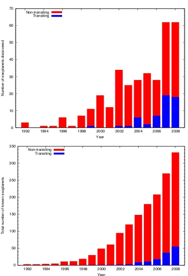
1.1 Discovery rate of extra-solar planets. . . 4

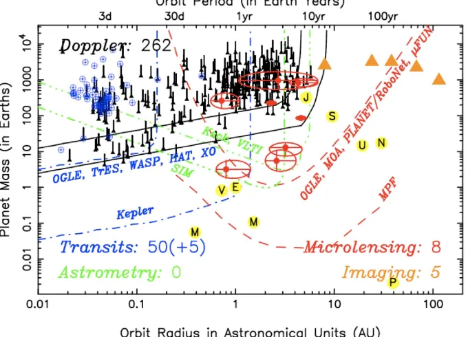
1.2 Exoplanet discovery space. Planet mass is plotted against orbital radius / or-bital period for 325 exoplanets. . . 5

1.3 Radial velocity curve of 51 Peg. . . 7

1.4 The 2004 June 08 transit of Venus across the Sun. . . 9

1.5 Transit photometry of HD 209458 b. . . 10

1.6 The SuperWASP observatories. . . 16

1.7 Mass-radius relation for extra-solar planets. . . 18

1.8 The 8.0µm secondary eclipse of TRES-1b. . . 19

1.9 Brightness of HD 189733 b. . . 20

2.1 RMS scatter versus magnitude for non-variable stars. . . 26

2.2 Cumulative distribution function of extra-solar planetary semi-major axis. . . 28

2.3 Transit depth versus magnitude for 329 simulated transiting extra-solar planets. 30 2.4 Signal-to-noise ratio versus magnitude for 329 simulated transiting extra-solar planets, for 51, 80 and 130 nights of data. . . 34

2.5 Transit detection efficiency as a function of period for fields with observations on 51, 80 and 130 nights. . . 35

2.6 Signal-to-noise ratio versus magnitude for 329 simulated transiting extra-solar planets, for 2 seasons each consisting of 130 nights of data. . . 36

2.7 Detection rate of transiting extra-solar planets versus number of nights of ob-servations. . . 36

3.1 HUNTER results for the planetary candidate 1SWASPJ060553.64+270837.7. . . . 42

3.2 Phase-folded lightcurves of 1SWASPJ060553.64+270837.7. . . 44

3.3 JGT images of 1SWASPJ060553.64+270837.7. . . 45

(15)

3.7 Photometry of 1SWASPJ211059.34+015711.9. . . 48

3.8 Partial transit lightcurve of 1SWASPJ211059.34+015711.9. . . 48

3.10 Partial transit lightcurve of 1SWASPJ062430.87+261906.0. . . 49

4.1 The predictions of Fortney et al. (2008) for the planetary radius that one would observe as a function of wavelength. . . 52

4.2 Flow chart describing the Metropolis-Hastings decision for a 1-dimensional model determined by the parameter, p. . . 54

4.3 Geometry of a planetary transit. . . 56

4.4 The distribution of values of the transit depth in the V-band produced by the DEPTHCOMcode. . . 61

4.5 Fitted transit depth for WASP-3 b against wavelength. . . 61

5.1 The probability that an outer planet transits, given that an inner planet with a period is observed to do so. . . 67

5.2 Plot indicating the maximum period for a planet to exhibit transits, as a func-tion of orbital inclinafunc-tion angle for a range of stellar masses. . . 71

5.3 Periodograms produced byHUNT1STARfor each of the 24 systems searched. . . . 76

5.4 Periodogram output ofHUNT1STARfor the unadulterated SuperWASP lightcurve of WASP-1. . . 77

5.5 Periodogram output ofHUNT1STARfor WASP-10. . . 78

5.6 Stellar rotation of WASP-10. . . 80

5.7 Detection criteria for simulated transits. . . 83

5.8 An example of an artificial transit which is successfully recovered in our simu-lations. . . 84

5.9 Simulation results (i) – WASP-1. . . 85

5.10 Simulation results (ii) – WASP-1. . . 86

5.11 Simulation results (iii) – selected planets. . . 91

5.12 Simulation results (iv) – WASP-1 at higher period resolution . . . 91

6.1 Series of time-stacked spectra for a typical pair of scans, ON and OFF. . . 100

6.2 Variance in the raw flux for the ON scans taken on 2007 April 23. . . 101

(16)

6.4 A typical ON scan of duration 120 s showing the raw counts (averaged over all frequency channels) as a function of time. . . 102

6.5 Uncalibrated lightcurves, ON and OFF, after subtraction of periodic RFI. . . 103

(17)

List of Tables

2.1 Fitted parameters for RMS scatter as a function of magnitude for the white and red noise cases . . . 29

2.2 The number of nights of observations for the three fields used in the signal-to-noise ratio analysis. . . 31

2.3 Simulated planetary detection rates. . . 37

4.1 The six parameters varied in theMCMCFIT code, and their prior distributions. . . 55

4.2 Initial standard deviation values for each proposal parameter. . . 59

4.3 The fitted depths of transit and associated 1-σuncertainties for WASP-3 b. . . . 60

5.1 Planetary systems searched for additional transiting bodies. . . 69

5.2 Best fitting parameters of a sine curve fitted to the lightcurve of WASP-10. . . 79

5.3 Model planet parameters used in simulations. . . 81

(18)

1

Introduction

1.1 Planets

1.1.1 Worlds beyond our own

There has been speculation about the possible existence of planets outside our Solar System

for many years. Famously, Giordano Bruno, later burned at the stake for heresy, postulated

the existence of extra-solar planets as part of his ‘infinite universe’ philosophy. In his De

L’Infinito Universo et Mondi (On the Infinite Universe and Worlds) of 1584, he declares his

belief (translation from Singer 1950) that,

"There are then innumerable suns, and an infinite number of earths revolve

around those suns, just as the seven we can observe revolve around this sun which

is close to us."

It took more than four centuries before the first of Bruno’s ‘infinite number of earths’

were discovered orbiting some of the ‘innumerable suns’ in our Galaxy. First, planets were

discovered orbiting pulsars Wolszczan & Frail (1992), and then, a few years later,

(19)

1.1. Planets

In the 14 years since Mayor & Queloz’s discovery of 51 Peg b, the pace of exoplanet

discovery has increased rapidly (Fig. 1.1).

1.1.2 The definition of a ‘planet’

Before going any further, it is useful to discuss exactly what is meant by the term ‘planet’. To

the ancient Greeks, the planets (meaning ‘wandering stars’) were the seven bodies thought

to orbit the Earth in the Ptolemaic system, namely the Moon, Mercury, Venus, the Sun, Mars,

Jupiter, and Saturn. After the heliocentric model of Copernicus became generally accepted,

the Moon and Sun were removed from the list of planets and the Earth added to the five

planets visible to the naked eye.

Although several of the larger main-belt asteroids were briefly classed as planets, the list of

known planets expanded slowly with the discoveries of Uranus in 1781 by Herschel (Herschel

& Watson, 1781), Neptune in 1846 by LeVerrier and Adams (Adams 1846; Le Verrier 1847),

and Pluto by Tombaugh in 1930 (Lowell Putnam & Slipher, 1932). The discovery of several

objects of similar size to Pluto orbiting the Sun beyond Neptune in recent years, combined

with the discovery of numerous planets orbiting stars beyond the Solar System, led to the

need for formal definitions of what constitutes a planet.

In 2003 the International Astronomical Union (IAU) adopted the following working

defi-nition of what constitutes anextra-solarplanet (Boss, 2003),

"1. Objects with true masses below the limiting mass for thermonuclear fusion

of deuterium (currently calculated to be 13 times the mass of Jupiter for objects

with the same isotopic abundance as the Sun) that orbit stars or stellar remnants

are "planets" (no matter how they formed). The minimum mass and size required

for an extrasolar object to be considered a planet should be the same as that used

in the Solar System.

2. Substellar objects with true masses above the limiting mass for

thermonu-clear fusion of deuterium are "brown dwarfs", no matter how they formed or

where they are located.

3. Free-floating objects in young star clusters with masses below the limiting

mass for thermonuclear fusion of deuterium are not "planets", but are "sub-brown

(20)

1.2. Discovering extra-solar planets

For the purposes of this thesis, and indeed any current work in the field of extra-solar

planets, the above definition is sufficient; there is no need for a lower limit to the mass.

The minimum mass required to constitute a planet is under debate within the context of

our own Solar System, but we are unable to discovery such low-mass objects around other

stars at present. Henceforth then, a ‘planet’, ‘exoplanet’, or ‘extra-solar planet’ will be used

interchangeably to mean an object less massive than 13 Jupiter masses (M_J), which is in orbit

around a star.

1.2 Discovering extra-solar planets

In this section, I outline briefly the history of exoplanet discovery and the different methods

used to detect such planets. The two most successful methods to date are the radial velocity

and transit methods; these methods are discussed in sections 1.2.2 and 1.2.3, respectively.

Pulsar timing (Sec. 1.2.1) was used to discover the first exoplanets, and gravitational

mi-crolensing (Sec. 1.2.4) and direct imaging (Sec. 1.2.5) have both been used successfully to

detect a number of planets. The less-successful methods of astrometry and transit timing are

also briefly discussed in Sec. 1.2.6 and Sec. 1.2.7, respectively.

1.2.1 Pulsar timing

The first extra-solar planets to be discovered were the low-mass planets orbiting the pulsar

PSR1257+12 (Wolszczan & Frail, 1992). They were discovered by measuring, with high

precision, the timing of this millisecond pulsar over several months. Because such objects

ordinarily have extremely stable rotation periods, it was possible for Wolszczan and Frail to

detect the variations in timing caused by the varying light travel time due to the reflex orbit

of the pulsar.

Although responsible for the first exoplanet discoveries, this method has only allowed the

discovery of a total of seven planets in four systems, and constitutes a separate line of study

to that of planets around main-sequence stars.

1.2.2 Radial velocity

By far the most successful of all planet-finding techniques to date is the radial velocity (RV),

or Doppler spectroscopy, method, which was responsible for all the planets discovered around

(21)

0 10 20 30 40 50 60 70

1992 1994 1996 1998 2000 2002 2004 2006 2008

Number of exoplanets discovered

Year Non-transiting

Transiting

0 50 100 150 200 250 300 350

1992 1994 1996 1998 2000 2002 2004 2006 2008

Total number of known exoplanets

Year Non-transiting

[image:21.595.116.504.105.674.2]

Transiting

Figure 1.1: Discovery rate of extra-solar planets. Upper panel: number of discoveries each year 1992

(22)

[image:22.595.144.484.249.494.2]

Figure 1.2: Exoplanet discovery space. Planet mass is plotted against orbital radius/orbital period

(23)

discovery of the first planet (OGLE-TR-56 b) by means of transits, in 2002 (Konacki et al.,

2003). Like the astrometric method (Sec. 1.2.6), the radial velocity method relies on detecting

the motion of a star around the barycentre of a planetary system. The RV technique allows

the velocity of the star along the line-of-sight to be determined, by measuring small changes

in the wavelength of stellar spectral lines caused by the Doppler effect. The amplitude of this

RV signal is proportional to the mass of the planet and inversely proportional to the square

of the orbital separation. This results in massive planets in close orbits being favoured by this

detection technique (see Fig. 1.2). Furthermore, because only the line-of-sight velocity can

be detected, systems that are inclined at close to 90◦_{, where the RV amplitude is maximal,}

are favoured. This also means that systems inclined at 0◦ _{cannot be detected as there is}

no component of the orbital reflex motion along the line-of-sight. In general, the orbital

inclination angle, i, is not known (unless i≈ 90◦_{, and the planet is observed to transit the}

disc of its host star, see Sec. 1.2.3) and so the planetary mass, M_p, cannot be determined

directly, onlyMpsini.

The orbital period, P, is determined directly from the radial velocity curve and the

eccen-tricity,e, of the orbit from the shape of this curve. Mpsiniis then calculated according to the

following equation (see e.g. de Pater & Lissauer 2001),

M_psini=K !

P

2πG "1

3#

M_∗ +M_p$

2

3%₁₋_e2 _, _(1.1)

where K is the semi-amplitude of the radial velocity signal andG the gravitational constant.

Since the stellar mass is several orders of magnitude larger than the planetary mass, the

approximation(M_∗ +M_p)_≈M_∗ can be used. The stellar mass is usually estimated from the

effective stellar temperature,Teff.

The amplitude of the radial velocity signal which revealed the presence of 51 Peg b is 59

ms−1_{, caused by a planet with} _M

psini = 0.47 MJorbiting a G5 dwarf in 4.23 d (Mayor &

Queloz 1995; Fig. 1.3). For comparison, Jupiter induces a reflex motion of 12.5 ms−1_{of the}

Sun, whereas the Earth produces only a 0.1 ms−1 _{shift. Sensitivity (rms) limits of 5 ms}−1 _for

10 yr and 1 ms−1 _{for 20 yr are indicated by black lines in Fig. 1.2. Current high-resolution}

spectrographs such as SOPHIE, which is in use on the 1.93-m telescope at the Observatoire

de Haute-Provence, can achieve Doppler spectroscopy with a stability of around 1–2 ms−1

(24)

[image:24.595.228.391.92.264.2]

Figure 1.3: Radial velocity curve of 51 Peg. The radial velocity of the star is plotted against the orbital

phase of the planetary system. Figure taken from Mayor & Queloz (1995)

1.2.3 Transits

It was seen in Sec. 1.2.2 that the information it is possible to obtain with the radial velocity

technique alone is limited. The orbital inclination angle remains unknown, and so only a

lower limit to the planetary mass is established. Detecting the reduction in stellar flux when

a planet passes directly in front of, or transits, its star allows the inclination angle to be

deter-mined (i=90◦for a star transiting the centre of its star). This, when combined with radial

velocity measurements, allows the mass of the planet to be determined. Transits also enable

the radius of the planet to be measured, allowing the mass-radius relation for these objects to

be investigated (Fig. 1.7). The amount of stellar light that is blocked by the passage of the

planet across the stellar disc is approximately equal to the square of the ratio of the planetary

and the stellar radii (see equation 1.5). Combining this with an estimate of the stellar radius

(e.g. from main-sequence stellar theory) allows a reasonably accurate determination of the

planet’s size. Transiting planets also allow all kinds of follow-up observations which mean

they can be characterised in ways not possible for non-transiting systems, as will be seen in

Sec. 1.5.

The obvious disadvantage of transits as a method of planet detection is that it requires

a fortuitous alignment of the system in order for a transit to be exhibited. For each

extra-solar planetary system that does exhibit transits, there will be many more that do not. The

probability,_&(alignment), that a particular planet transits its host star can be calculated from

consideration of the geometry of the system (assuming orbits that are randomly inclined to

(25)

In order for a system to exhibit transits, the following condition must be satisfied (Sackett,

1999),

cosi≤R∗+Rp

a , (1.2)

whereR_∗ is the stellar radius,Rp the planetary radius, anda the orbital semi-major axis.

The probability that a given system transits can be calculated by integrating over the values

of cosi that result in a transit and normalising by the integral of all possible values of cosi,

which are equally likely if planetary orbits are randomly inclined to the line-of-sight,

&(alignment) =

&(R_∗+Rp)/a

0 d(cosi) &1

0 d(cosi)

= R∗+Rp

a ≈

R_∗

a (1.3)

Thus the probability of a Solar System analogue being aligned such that Earth transits the

Sun is 0.0046, and for Jupiter this probability is 0.0001. Also, several transits of a particular

object must be observed in order to confirm the existence of a planet, requiring that

observa-tions be made over a time-scale equal to several times the orbital period. The gap between

observations must be less than the duration of the transit, in order not to miss such an event.

The duration of transit,ttris a function ofR∗,a and the orbital period,P,

ttr= R_∗P

πa , (1.4)

assuming a circular orbit and an equatorial transit. The duration of a Jupiter transit is

there-fore around 1.2 d, and an Earth transit would last for around 13 h.

The reduction in brightness (depth) of the host star during transit,∆m, is proportional to

the ratio of the squares of the radii of planet and star. Tingley & Sackett (2005) determine

the depth to be given by,

∆m_≈1.3 !_R

p R_∗

"2

(1.5)

The factor of 1.3 in this equation arises from modelling the limb-darkening of the star, i.e.

it accounts for the fact that the stellar disc is not uniformly bright, but is darker around the

edges (limbs). The transit depths for Earth and Jupiter transiting the Sun are 0.01 and 1.3

(26)

[image:26.595.236.388.93.240.2]

Figure 1.4:The 2004 June 08 transit of Venus across the Sun. Photograph taken from JBAA (2005)

in 2004, producing a transit with a depth fractionally shallower than that produced by an

Earth-sized planet.

All of the above results in the requirements that, even if every star had an Earth analogue,

we would have to observe around 200 such systems to detect a single Earth. The observations

would have to made with the precision of the order of tens of micro magnitudes, continuously

for several years. Current ground based photometric precision is of the order of 1 mmag.

Much easier to find, however, are transiting hot Jupiters (HJs). These typically have

periods of just a few days; separations of a few hundredths of an astronomical unit; and

transit durations of a few hours1_{. Additionally, the probability of alignment such that transits}

will occur is much greater for a HJ system than for planets that orbit at several au. For a

typical HJ,_&(alignment)_≈0.1; that is about 1 in 10 HJs will exhibit transits.

HD 209458 b: the first transiting planet

Although transits were proposed as a means for detecting planets similar to hot Jupiters by

Struve (1952) (who also suggested the use of high-precision radial velocity measurements to

detect planets), the first exoplanet detected by means of transits was HD 209458 b, which

had already been discovered by radial velocity observations. Transits of this system were

observed by Charbonneau et al. (2000) and by Henry et al. (2000). The transits observed

by Charbonneau et al. (2000) using STARE, a small (0.1-m), wide-field survey telescope are

compared in Fig. 1.5 to the high-precision photometry later obtained by Brown et al. (2001)

using theHubble Space Telescope.

Because of the proximity to Earth of HD 209458 and its consequent brightness (it remains

1_{Take, for instance, the first known transiting exoplanet HD 209458 b, which has} _P₌_{3.52 days;}_a₌_{0.045 au;}

(27)

Figure 1.5: Transit photometry of HD 209458 b. Left: The first ever exoplanet transit lightcurve,

taken with theSTAREtelescope. Figure taken from Charbonneau et al. (2000). Right: AHubble Space Telescopelightcurve taken from Brown et al. (2001).

the brightest transiting planet host star, with V = 7.65), HD 209458 b remains a popular

target for various follow-up observations and characterisation studies (see Sec. 1.5 for some

examples).

Transit surveys

The discovery of the transits of HD 209458 b inspired a plethora of surveys to detect planets

using transits in the first instance. These surveys have become increasingly successful over

the past few years, and are responsible for all but six of the known transiting planets to date2.

Fig. 1.1(a) shows the increasing proportion of known planets that transit their host stars.

As a further illustration of the recent rate of exoplanet discovery, when the work for this thesis

commenced in 2005 September, only 10 transiting planets were known, this number now

stands at 59. In the same time, the total number of known exoplanets has doubled to 348 (as

at 2009 May).

The transit surveys employed to date fall into one of three categories of survey, (i)

wide-field surveys using similar types of camera to that Charbonneau et al. (2000) used to detect

the transits of HD 209458 b; (ii) deep surveys using larger (typically_∼2 m in diameter), more

conventional telescopes; and (iii) space-based endeavours such asCoRoT(Barge et al., 2008)

andKepler(Borucki et al., 2009), which represent the next generation of transit surveys.

The Optical Gravitational Lensing Experiment (OGLE), a deep field survey, was initially

the most successful, with five discoveries between 2002 and 2004 (as well as a further three

in 2007). However, the faint nature of stars in such a deep survey (the OGLE planet host stars

2_{HD 149026 b, HD 17156 b, HD 189733 b, HD 80606 b and GJ 436 b were, like HD 209458 b, initially detected}

(28)

all have I-band magnitudes between 14 and 16) make spectroscopic confirmation difficult,

and preclude much follow-up work as well. They do, rather like gravitational microlensing,

however, offer insight into the frequency of planets around stars beyond the immediate Solar

neighbourhood in the Galaxy.

The wide-field surveys have been the most successful, not only in quantitative terms

(re-sponsible for 35 of the 59 known transiting exoplanets), but also in providing targets for

char-acterisation work (see Sec. 1.5). Several similar wide-field surveys are in successful operation,

namely HATNet (Hungarian Automated Telescope Network) (Bakos et al., 2002); Super-WASP

(Wide Angle Search for Planets) (Pollacco et al. 2006; Sec. 1.3); TrES (Trans-Atlantic

Exo-planet Survey), which incorporates the aforementioned STARE telescope (O’Donovan et al.,

2006b) and XO (McCullough et al., 2005).

These wide-field survey instruments typically consist of a battery of small lenses, each

equipped with a CCD camera which images tens of square degrees, operated robotically. Large

numbers of stars are imaged many times per night, and the resulting lightcurves are searched

for transit signatures. Once these transiting planet candidates are identified, follow-up

ob-servations, in the form of Doppler spectroscopy measurements, are required to confirm the

planetary nature of the transiting body. Higher-precision transit photometry is usually

ob-tained as well, in order to better constrain observational parameters such as the transit depth

and duration, leading to more accurate measures of parameters such as the planetary radius.

The operation of wide-field transit surveys will be discussed in greater detail in Sec. 1.3,

with specific reference to the SuperWASP survey, and the subject of follow-up photometry is

discussed further in Chapter 3.

Although the wide-field surveys have reached maturity over the last few years and are now

operating in what Charbonneau (2009) describes as ‘production-line mode’, the exoplanet

discovery space that they can explore remains limited (Fig. 1.2). The factors limiting the

ability to find longer-period planets are, of course, the length of the observing baseline, and

the transit probability (Eqn. 1.3). The ability to find longer-period planets will increase with

time if such surveys continue to observe the same fields (see chapter 2), although data sharing

between survey instruments at different longitudes may be required to maximise the planet

haul in the presence of the problem of observing windows (Fleming et al., 2008). That is,

(29)

planets with certain ephemerides will never be observed to transit from a particular terrestrial

longitude.

Pushing down the limit to the size of planets that wide-field transit surveys can find

per-haps represents a bigger problem, determined as it is by the precision of the photometry. It

may prove possible to achieve higher-precision photometry, however, as the sources of

system-atic noise inherent in all these surveys becomes better understood and strategies are

devel-oped to reduce it. As is demonstrated in chapter 2, observing a given system for longer (and

thus observing a greater number of individual transits) acts to increase the signal-to-noise

ratio and so make smaller transits detectable.

The potential improvements in wide-field surveys described in the previous paragraph will

still prove insufficient to enable these surveys to detect Earth-like planets around Solar-type

stars, which is regarded by many as one of the major goals of exoplanet discovery. Wide-field

surveys may, however, discover planets at orbital distances at which liquid water may exist on

the planetary surface. The range of orbital distances for which this is the case is known as the

‘habitable zone’ of a star (Kasting et al., 1993), the location of which varies with the spectral

type of the star. Because M-dwarfs have much smaller luminosities than G-dwarfs such as

the Sun, the habitable zone is located much closer to the star, reducing the orbital period

of planets in the habitable zone, as well as increasing the geometric probability of transit.

Furthermore, because of the much smaller radius of these stars, much smaller planets can be

discovered for a given photometric precision.

Charbonneau (2009) considers the case of a planet with a radius twice that of Earth

orbiting in the habitable zone of both a G2-dwarf and an M5-dwarf. The planet orbits the

G2-dwarf with a period of 1 yr and a transit probability of around 0.5 per cent, compared to

just 15 d in the case of the M5-dwarf with a transit probability of 1.6 per cent. The depths of

the two transits would be 0.03 and 0.5 per cent respectively. The radial velocity signal is also

more favourable in the M-dwarf scenario; the peak-to-peak amplitude is 10ms−1 _compared

to 1.3ms−1_{for a planet of mass 7}_M

⊕. The next generation of ground-based surveys, such as

MEarth(Irwin et al., 2009) may discover the first ‘habitable’ exoplanets, or that honour may

fall to a space-based mission.

Going into space removes many of the sources of systematic noise that afflict

(30)

as the recently launched Kepler(Borucki et al., 2009) andCoRoT (Convection Rotation and

planetary Transits; Barge et al. 2008) aim to find smaller planets than those discovered by

ground-based surveys.

1.2.4 Gravitational microlensing

When one star passes behind another, the foreground star may act as a gravitational lens,

bending light from the background star, resulting in magnification of the background star.

This gravitational microlensing effect was predicted by Einstein (1936) and later suggested

as a means of exoplanet discovery by Mao & Paczynski (1991). If the lens star is host to an

orbiting exoplanet, the planet may cause a secondary magnification of the background source,

and detailed modelling of the resulting lightcurve allows, for example, determination of the

mass-ratio of the system. The first planet to be discovered in this manner was a 1.5MJplanet

in a_∼3 au orbit (Bond et al., 2004), and the method is responsible, as of 2009 June, for the

discovery of a total of eight exoplanets in seven systems3.

Microlensing allows planets to be discovered around stars which lie much further from

Earth than those discovered by other methods (_∼ 1000 pc compared to _∼ 100 pc), indeed

recent work by Ingrosso et al. (2009a) suggests that it may be possible to find exoplanets

beyond our Galaxy, in M31, using microlensing. Microlensing also probes a different area of

exoplanet parameter space, able to find low-mass planets at large orbital separations (Fig.

1.2).

The greatest drawback of the method is that the detection of a planet around the lens star

is only possible during the unique microlensing event. The host star is distant and faint, so it is

not currently possible to gain any further information about such systems from spectroscopic

or photometric measurements.

1.2.5 Direct imaging

Attempting to image directly an extra-solar planet poses a significant technical challenge;

planets are generally 106 to 1012 times fainter than their host stars and are typically sepa-rated by angles of less than 1 arcsecond, even for nearby systems (Beuzit et al., 2007). Direct

imaging favours companions that are young and therefore still warm, large, and which

or-bit reasonably far from a small star. Early successes include the imaging of a 5 M_Jplanet

(31)

orbiting a brown dwarf at 55 au (Chauvin et al. 2004, 2005). More recently, planets have

been imaged around earlier-type stars, such as the discovery of a planet orbiting the nearby

(7.7 pc) A-dwarf Fomalhaut at a distance of 119 au (Kalas et al., 2008). Marois et al. (2008)

succeeded in imaging a system of three planets, with masses between 5 and 13 M_J, around

HR 8799. They used adaptive optics (AO) to increase the spatial resolution of the images from

the limits imposed by the atmosphere, towards those imposed by diffraction. Angular

differ-ential imaging (ADI) was also used to distinguish between exoplanets and optical artefacts

by allowing the field-of-view to rotate around the star as the telescope tracked the target. To

date, a total of eleven planets in nine systems have been imaged. Future instruments such as

SPHERE (Spectro-Polarimetric High-contrast Exoplanet REsearch; Beuzit et al. 2008) and GPI

(Gemini Planet Imager; Graham et al. 2007) will extend our ability to image planets closer to

their stars.

1.2.6 Astrometry

Astrometry has long been suggested as a potential method for discovering exoplanets. Like

the RV method (Sec. 1.2.2), it relies on the fact that star and planet orbit a common

centre-of-mass and a sufficiently centre-of-massive planet will cause the movement of its star to be large enough

to be measurable. Instead of measuring the movement of the star along the line of sight

(like the RV method), astrometry measures the movement of the star in the plane of the sky.

Unlike the RV method, however astrometry favours long-period planets Sozzetti (2005). This

is because, with astrometry, it is easiest to measure a large orbital reflex displacement, rather

than a large orbital reflex velocity, which is preferred by RV.

Several claims to have detected planets via astrometry have been made, almost all of

which have later been retracted or discredited. Perhaps most notorious was the announcement

of the discovery of two extra-solar planets around nearby Barnard’s star by van de Kamp

(1969), which have never been confirmed.

More recently, Benedict et al. (2002) used astrometry to measure the mass of the exoplanet

Gl 876 b, already known by RV. The combination of astrometry and radial velocity enables the

orbital inclination angle to be determined, and thus the true planetary mass. As Tuomi et al.

(2009) suggest, high-precision astrometric measurements can be complementary to radial

(32)

1.3. SuperWASP

Even more recently, Pravdo & Shaklan (2009) report what could, if confirmed, represent

the first discovery of an exoplanet by means of astrometry. The putative planet has a mass of

6.4M_Jand it resides in a 0.74 yr orbit around the nearby ultra-cool dwarf star, VB 10.

1.2.7 Transit timing

Although no planets have yet been discovered by means of transit timing variations (TTV),

the method provides an opportunity to discover multiple planet systems (see Chapter 5) and,

potentially, Earth-mass planets. The times of transit of a known transiting planet can be

altered by the influence of an additional planet in the system (Agol et al. 2005; Holman &

Murray 2005). The TTV method is particularly sensitive to planets in resonant orbit with the

transiting planet; such resonant planets are detectable even if they are of very low mass.

1.3 SuperWASP

1.3.1 Instruments

SuperWASP is a consortium comprising members at Queen’s University Belfast, the University

of St. Andrews, the University of Leicester, Keele University, the Open University, the Isaac

Newton Group of telescopes, the University of Cambridge, and the Instituto de Astrofísica

de Canarias4_{. This consortium operates two robotic observatories, which are employed as}

wide-field transit surveys (see Sec. 1.2.3). The first observatory, SuperWASP-N, is located

in the Northern hemisphere, at the Observatorio del Roque de los Muchachos on the island

of La Palma in the Canaries. The second, WASP-South, is in the Southern hemisphere, at

the South African Astronomical Observatory near Sutherland in the Republic of South Africa.

SuperWASP-N commenced observations in 2004, followed by WASP-South in 2006.

Each SuperWASP installation comprises an array of eight5 200mm f/1.8 Canon camera lenses, each with a 4 mega-pixel CCD recording a 7.8◦ _{by 7.8}◦ _{field (Pollacco et al., 2006).}

These eight cameras are mounted on a fork mount, which is housed in an enclosure with a

hydraulically operated roof (Fig. 1.6), which also houses a weather station.

4_{SuperWASP website – http:}_//_{www.superwasp.org}

(33)

1.3. SuperWASP

Figure 1.6: The SuperWASP observatories. Left: The enclosure of SuperWASP-N on La Palma. Right:

The eight cameras of WASP-South in South Africa. Photographs taken from the SuperWASP website – http://www.superwasp.org

1.3.2 Observations

The SuperWASP observing strategy is designed to maximise the number of stars that can be

hunted for transits, without introducing large numbers of blended objects, which can be a

problem given the large pixel size of 13.7))_{. For this reason, overcrowded fields near the}

galactic plane are avoided (Christian et al., 2005). The sky is tiled in right ascension, with up

to 8 fields being observed at a time. Around a minute is spent on each field, including a 30

s exposure, 4 s of read-out time, and slewing, giving photometry with a cadence of about 8

minutes.

1.3.3 Data reduction

Since each SuperWASP exposure generates an 8.4 Mb image file, a large quantity of data is

stored and processed; this is done using a custom-written data reduction pipeline (Pollacco

et al., 2006). The pipeline uses the Tycho 2 and USNO B catalogues to prepare an astrometric

solution for each field. Aperture photometry is performed on all objects, using three different

sized apertures and airmass and CCD position trends are removed from the data before it is

archived at the University of Leicester (Pollacco et al., 2006).

Prior to searching the data for transits, the SYSREM algorithm of Tamuz et al. (2005) (see

Chapter 2) is applied to the data to reduce systematic errors. Four components of systematic

error are removed with SYSREM; it is thought that two of these are caused by airmass

(34)

1.4. Multiple planet systems

(Collier Cameron et al., 2006). The HUNTERalgorithm of Collier Cameron et al. (2006), which

is an adaptation of the box least-squares method (Kovács et al., 2002), is used to search the

data for transit-like signatures.

Photometric followup (Chapter 3) and Markov-chain Monte Carlo analysis (Chapter 4)

are used to further characterise the resulting planetary candidates, and to eliminate various

types of astrophysical false-positive. Candidate planets surviving these and various statistical

tests, are then observed with Doppler spectroscopy to confirm that the transit is caused by an

object of planetary mass (see e.g. Cameron et al. 2007; Sec. 1.2.2).

1.4 Multiple planet systems

Of the 349 known exoplanets (to 2009 June 08), 91 are known to reside in a total of 37

multiple planet systems6_{. Multiple planet systems are of particular interest for a number of}

reasons. They are of interest as comparisons to the Solar System, allow multi-body dynamical

studies and constrain models of planet formation. Furthermore, additional planets may be

detected by their actions on an already known planet, in the same way as Neptune was

dis-covered through its perturbations on the motion of Uranus. The transit-timing method (Sec.

1.2.7) is an example of a method for detecting multiple planets which is complementary to

other methods, and has a greater sensitivity to low-mass planets than other methods do at

present.

The significance of multiple planet systems in which one or more of the planets exhibits

transits is discussed in Chapter 5, along with a description of the various methods proposed

to detect such systems.

1.5 Characterising transiting extra-solar planets

As mentioned in Sec. 1.2.3, measurements of transiting planets, in combination with radial

velocity data, allow the determination of planetary masses and radii. The discovery of over

fifty transiting planets allows the construction of an observational mass-radius diagram (Fig.

1.7). This illustrates the huge variation in mean density for planets of a similar size, the cause

of which is, at present, poorly understood; it is not possible to predict whether a given planet

will be ‘inflated’ or not (Charbonneau, 2009). Efforts have been made to model the structure

(35)

1.5. Characterising transiting extra-solar planets

0 0.5 1 1.5 2

0 0.5 1 1.5 2 2.5 3 3.5 4

Radius / Jupiter radii

Mass / Jupiter masses

ρ = 300 kg m-3

ρ = 600 kg m-3

ρ = 1000 kg m-3

ρ = 1500 kg m-3

[image:35.595.114.505.92.375.2]

ρ = 3000 kg m-3

Figure 1.7: Mass-radius relation for extra-solar planets. 53 transiting planets with masses less than

4MJare shown (black circles), along with Jupiter (black triangle) and Saturn (orange square). Also shown are lines of constant mean density.

and formation of these hot Jupiters, however, and it is data from transiting planets that will

be required to understand fully this issue.

Beyond exploring the structure and formation of exoplanets, transiting planets allow

char-acterisation of their atmospheres without the requirement that we image the planets directly.

These techniques exploit the fact that the planet passes directly in front of the star and that,

half an orbit later, the planet passes behind the star in secondary eclipse.

Transmission spectra can be used to identify various components of the planetary

atmo-sphere. By subtracting spectra of the star taken in and out of transit, features caused by

absorption in the planetary atmosphere can be identified. This technique has been used to

detect, for instance, the presence of sodium in the atmosphere of HD 209458 b

(Charbon-neau et al., 2002), as well as water (Tinetti et al., 2007) and methane (Swain et al., 2008)

molecules in the atmosphere of another transiting exoplanet, HD189733 b.

The Spitzer space telescope has been used to detect the secondary eclipse of a number

of exoplanets at infra-red wavelengths. The detection of the secondary eclipse of TrES-1 by

(36)

extra-1.6. Star - planet interaction

Figure 1.8: The 8.0µm secondary eclipse of TRES-1b. The solid lines is the best-fitting model which

has a depth of 0.00225 and a timing offset (from phase 0.5) of+8.3 min. The dashed line is the same, but for a timing offset of zero. Figure taken from Charbonneau et al. (2005).

solar planet, and also allowed the albedo of the planet to be estimated (Fig. 1.8). Spitzer

data also enabled Knutson et al. (2007) not only to measure the temperature, but to map the

distribution of temperatures as a function of planetary longitude (Fig. 1.9).

1.6 Star - planet interaction

Recent studies of hot Jupiter planetary systems have revealed that the star and planet can

interact both magnetically and tidally (see e.g. Shkolnik et al. 2009). Through magnetic

in-teractions, the planet can induce activity in the photosphere and upper atmosphere of the star.

Tidal interactions commonly result in the planet rotation period and orbital period becoming

synchronised.

1.6.1 Low-frequency radio emission from exoplanets

The magnetic field strength of an exoplanet has not yet been measured, but this is thought to

be possible through detection of low-frequency radio emission from the planet. Such emission

is predicted to occur as a result of magnetic interactions between star and planet, in a manner

(37)

1.6. Star - planet interaction

Figure 1.9: Brightness of HD 189733 b. Estimated brightness, assuming the planet is tidally locked,

(38)

1.7. Overview of thesis

at frequencies of about 30 MHz; this is caused by charged particles from the solar wind

interacting with the planetary magnetosphere, resulting in the emission of electron-cyclotron

maser emission (see Sec. 6.1 for a more detailed discussion of this).

1.7 Overview of thesis

What follows is a brief description of the content of each of the major chapters of this thesis:

• In chapter 2, I investigate correlated ‘red’ noise as an explanation for why wide-field

transit surveys have not yielded the number of planets originally predicted. The stellar

populations in the fields observed by one of the SuperWASP-N cameras in the 2004

observing season are modelled. The number of planets detectable in the presence of red

noise is predicted.

• An overview of follow-up photometry to SuperWASP observations is presented in

chap-ter 3. Examples are used to illustrate some of the possible outcomes of follow-up

pho-tometry.

• In chapter 4, I describe the development of two Markov-Chain Monte Carlo (MCMC)

codes which fit models to transit lightcurves, with the aim of measuring any variation

in transit depth with wavelength.

• Chapter 5 is a description of a search of archive SuperWASP photometry for additional

transiting planets in known planetary systems. The rotation of a planet host-star is

investigated and the ability of SuperWASP to find multiple planet systems is quantified.

• In chapter 6, the first attempt to detect the secondary eclipse of a transiting exoplanet

at radio wavelengths is reported. Observations of HD 189733 b are interpreted in the

context of electron-cyclotron maser emission, which is predicted to occur when an

exo-planetary magnetic field interacts with the stellar wind.

• Finally, the major findings of the previous chapters are summarised in chapter 7, and

(39)

2

The impact of correlated noise on SuperWASP

detection rates

This chapter is based on an article published inMonthly Notices of the Royal Astronomical

Society:

Smith, A. M. S., Collier Cameron, A., Christian, D. J., Clarkson, W. I., Enoch, B., Evans, A.,

Haswell, C. A., Hellier, C., Horne, K., Irwin, J., Kane, S. R., Lister, T. A., Norton, A. J., Parley, N.,

Pollacco, D. L., Ryans, R., Skillen, I., Street, R. A., Triaud, A. H. M. J., West, R. G., Wheatley, P.

J., & Wilson, D. M., ‘The impact of correlated noise on SuperWASP detection rates for transiting

extra-solar planets’, 2006, MNRAS, 373, 1151.

All the work described here was conducted by the author.

In this chapter I present a model of the stellar populations in the fields observed by one of

the SuperWASP-N cameras in the 2004 observing season. I use the Besançon Galactic model

Above: The five cameras which comprised SuperWASP-N, at the Observatorio del Roque de los Muchachos on La

(40)

2.1. Introduction

to define the range of stellar types and metallicities present, and populate these objects with

transiting extra-solar planets using the metallicity relation of Fischer & Valenti (2005). The

ability of SuperWASP to detect these planets in the presence of realistic levels of correlated

systematic noise (‘red noise’) is then investigated.

2.1 Introduction

Transit surveys have the potential to find numerous hot Jupiter-like planets (HJs), that is

Jupiter-sized planets which orbit close to their host star with periods of just a few days. The

probability that a HJ system is aligned such that transits will occur is about 0.1; which is

much more favourable than planets orbiting at greater distances (for an Earth-like orbit, the

probability of transit alignment is 0.0046).

Previous attempts have been made to estimate the expected detection rates of transiting

HJs by shallow, wide-field transit surveys similar to SuperWASP (e.g. Brown 2003). Based

on an observing pattern consisting of 38 nights of observations spread over 91 days and a

requirement that three or more transits are observed, Brown calculated the detection rate of

HJs producing a transit of depth 1 per cent or greater to be 0.39 per 104 _{stars. Brown also}

estimates that, for the same observing window function, 4.51 false alarms will be detected

per 104 _{stars – indicating that only eight per cent of transit signals detected will be produced}

by planets. These planetary transit ‘impostors’ are grazing eclipsing binaries and eclipsing

binaries diluted by light from a third star (either a field star or the third member of a triple

system).

The SuperWASP survey has the potential to define the population of extra-solar planets

which transit nearby bright stars (V < 13). In order for the results of SuperWASP to be

properly interpreted, it is essential that the selection effects that operate in the survey are

well understood. In this work, I use the findings of Pont (2006) and Pont, Zucker & Queloz

(2006) to estimate SuperWASP’s detection rate in the presence of realistic levels of systematic

red noise. I find that in order to detect a significant number of transiting planets, the existence

(41)

2.2. Observations

2.2 Observations

Observations were conducted with SuperWASP-N (Sec. 1.3) during 2004, when the

instru-ment was operated using only five cameras. The data were reduced in the standard manner

described in Sec. 1.3, and the usual four components of correlated noise (one caused by

airmass, one by thermal induced focus variations) are removed by the SYSREM algorithm of

Tamuz et al. (2005).

2.3 ‘Colours’ of noise in photometric data

Pont (2006) demonstrated that there is likely to be significant co-variance structure in the

noise in data from ground-based photometric surveys, such as SuperWASP. Previous forecasts

of the planet ‘catch’ from such instruments (e.g. Horne 2001) have assumed that such noise

is un-correlated or ‘white’ in nature. Pont et al. suggest that the reduced signal-to-noise

caused by correlated or ‘red’ noise can account for an observed shortfall in transiting planet

detections.

Noise consisting of white, independent, random noise combined with red, co-variant,

sys-tematic noise is termed ‘pink’. Unlike white noise, this cannot be removed by averaging the

data if the noise is on the time scale of the transits we wish to detect. Pont (2006) showed that

systematic noise, correlated on time scales equivalent to a typical hot Jupiter transit (≈ 2.5

hours) cannot be ignored and indeed tends to be the dominant type of noise for bright stars.

It therefore seems likely that the noise in SuperWASP data will be pink.

2.4 Characterisation of SuperWASP noise

The simplest method of establishing the level of correlated noise present in the data is to

compute a running average of the data over the n data points contained in a transit-length

time interval (Pont et al., 2006). The transit duration chosen here is 2.5 hours, which is the

transit duration corresponding to a planet orbiting a solar analogue, with a period of 2.6 days

– typical of a hot Jupiter. Since exposures are taken at roughly 7 minute intervals, there are

aboutn=20 points in each interval.

If the noise is purely random, the RMS scatter in the average ofndata points should be

(42)

2.5. Simulated planet catch

systematic component in the noise, the RMS scatter of the average ofnpoints will be greater

than this.

The RMS scatter,σ, is calculated for each of the 822 stars determined to be non-variable

in the field centred at 15h17min RA,+23◦₂₆)_{dec for which lightcurves have been produced}

by the SuperWASP data reduction pipeline. The noisiest 25 per cent of the data points in each

lightcurve, corresponding to measurements made around full moon and during Sahara dust

events, are excluded from the analysis. Stars are determined to be variable, and excluded

from the analysis, if%σ2_s >0.005 mag, whereσ2_s is the variance caused by intrinsic stellar variability, derived from theχ2statistic for a constant-flux model.

The running average,σr, over 20 points is also calculated for each of these stars, with the

same exclusions of the noisiest data and intrinsically variable stars.

Bothσw andσrare calculated prior to, and after, some red noise has been removed with

SYSREM. These quantities, andσ, are plotted against magnitude for the 822 non-variable stars in the field in Fig. 2.1.

As indicated by the differences between Figs. 2.1(a) and 2.1(b), the SYSREM algorithm is

highly effective at reducing the levels of systematic noise present in the data. Fig. 2.1(b) also

shows, however, that not all correlation in the noise is removed by SYSREM. If that were the

case, the σr curve would lie over the σw curve. Instead, the σr curve lies higher than σw,

and flattens out at about 3 mmag for bright (V=9.5) stars, indicating that systematic trends

of this magnitude are present in the data on a 2.5 hour time-scale.

2.5 Simulated planet catch

I model the objects in the 36 fields viewed by one of the SuperWASP cameras in the 2004

season, by using the Besançon model of the Galaxy (Robin et al., 2003) to generate a star

catalogue of stars with 9.5<V <13.0 for each of the fields. Planets are then assigned to stars

that are of spectral class F, G or K and luminosity class IV or V on the basis of their metallicity,

using the planet-metallicity relation of Fischer & Valenti (2005):

(43)

0.001 0.01 0.1

9.5 10 10.5 11 11.5 12 12.5 13

RMS scatter (magnitude)

WASP V magnitude

(a) Before decorrelation with SYSREM

0.001 0.01 0.1

9.5 10 10.5 11 11.5 12 12.5 13

RMS scatter (magnitude)

WASP V magnitude

(b) After decorrelation with SYSREM

Figure 2.1:RMS scatter versus magnitude for non-variable stars in the field centred at 15h17min RA,

(44)

where &(planet) is the probability that a particular star of metallicity [Fe/H] is host to a

planet. The above equation is used for stars which have metallicities in the range -0.5<[Fe/H]<0.5.

For stars with[Fe/H]_{< −}0.5,_&(planet) = 0.003, and for[Fe/H]>0.5,&(planet) =0.3.

Only stars of spectral type F, G and K are allocated a non-zero planet hosting probability,

since the Fischer & Valenti (2005) equation is based upon radial velocity observations of stars

of this type only. This does not pose a significant problem, however, as early-type stars are

not numerous and have radii that are too great for transit detection. M-type stars are not

particularly numerous in the Besançon-generated catalogues either (about 2.8 per cent of

the stars are of type M or later), because the sample is limited by apparent magnitude, not

volume. Although the transit signal produced by a Jupiter-like planet orbiting an M dwarf

star will be greater than that produced by, say, a G dwarf star, M dwarfs are thought to be less

likely to harbour giant planets (Adams et al., 2005). Similarly, only subgiants and dwarfs are

considered planet hosts, since any planet orbiting a giant star would produce an insufficiently

deep transit signature to be detected.

The probability that a star hosts a transiting planet is calculated using

&(transit) =_&(planet)_{× &}(alignment) (2.2)

where&(alignment)is the probability of a given planetary system being aligned with respect

to the line of sight such that a transit can be observed. As it was shown in Sec. 1.2.3, this is

given by

&(alignment) = R∗ +Rp

a ≈

R_∗

a (2.3)

whereR_∗ is the stellar radius,R_p the planetary radius andathe semi-major axis of the system.

The semi-major axis of each potential planetary system in the model is drawn randomly from

a distribution that is uniform in log (a), between 0.02<a<5.25 au.

This simple log-flat distribution of semi-major axes is compared to the actual distribution

ofaamongst extra-solar planets discovered by Doppler surveys in Fig. 2.2. Our distribution

appears to be a poor fit to the observed distribution in the regime favoured by transit surveys

(a ! 0.05 au), which may lead to an overestimation of the number of very short-period

planets. The distributions, however, closely agree on the fraction of planets witha_≤0.05 au

(45)

0 0.2 0.4 0.6 0.8 1

0.01 0.1 1 10

Cumulative distribution function

Semi-major axis (au)

Figure 2.2:Cumulative distribution function of extra-solar planetary semi-major axis. The filled circles

represent the 186 planets discovered by radial velocity means, as at 2006 September 15. The solid line is the distribution (uniform in log (a) for 0.02 < a < 5.25 au) used in our model.

gives 16 per cent.

On the basis of the probability_&(transit), for each star, it is determined whether or not a

star hosts a transiting planet. It is assumed, for simplicity, that all planets have a radius,Rp,

equal to that of Jupiter, R_J. The depth of transit, ∆m, is determined from the equation of

Tingley & Sackett (2005),

∆m_≈1.3 !_R

p R_∗

"2

(2.4)

The factor of 1.3 in the above equation takes account of the effect of stellar limb-darkening,

and although this assumes a central transit, off-centre transits will only have a slightly smaller

limb-darkening factor (Tingley & Sackett, 2005).

A total of 355,429 stars are generated by the Besançon model in the 36 fields, 165,586

(46.6 per cent) of which are of type F,G or K and class IV or V. The simulation described above

results in the allocation of a transiting planet to 329 of these stars, although this number

changes each time the simulation is run because it relies on random numbers (see §2.6.2 for

discussion of this). The transit depths of these 329 systems are calculated using equation 2.4.

Searching for transiting extra solar planets at optical and radio wavelengths

SEARCHING FOR TRANSITING EXTRA-SOLAR PLANETS AT

OPTICAL AND RADIO WAVELENGTHS

Alexis Michael Sheridan Smith

A Thesis Submitted for the Degree of PhD

at the

University of St. Andrews

2009

Full metadata for this item is available in the St Andrews

Digital Research Repository

at:

https://research-repository.st-andrews.ac.uk/

Please use this identifier to cite or link to this item:

http://hdl.handle.net/10023/871

Searching for Transiting Extra-solar Planets at

Optical and Radio Wavelengths

Alexis Michael Sheridan Smith

Submitted for the degree of Doctor of Philosophy

Declaration

Copyright Agreement

Abstract

Acknowledgements

Contents

List of Figures

List of Tables

1

Introduction

1.1

Planets

1.1.1

Worlds beyond our own

1.1.2

The definition of a ‘planet’

1.2

Discovering extra-solar planets

1.2.1

Pulsar timing

1.2.2

Radial velocity

1.2.3

Transits

1.2.4

Gravitational microlensing

1.2.5

Direct imaging

1.2.6

Astrometry

1.2.7

Transit timing

1.3

SuperWASP

1.3.1

Instruments

1.3.2

Observations

1.3.3

Data reduction

1.4

Multiple planet systems

1.5

Characterising transiting extra-solar planets

1.6

Star - planet interaction

1.6.1

Low-frequency radio emission from exoplanets

1.7

Overview of thesis

2

The impact of correlated noise on SuperWASP

detection rates

2.1

Introduction

2.2

Observations

2.3

‘Colours’ of noise in photometric data

2.4

Characterisation of SuperWASP noise

2.5

Simulated planet catch