Search with Evolutionary Ruin and Stochastic Rebuild: a Theoretic Framework and a Case
Study on Exam Timetabling
Jingpeng Li* Ruibin Bai
Division of Computing Science & Mathematics Division of Computer Science University of Stirling The University of Nottingham Ningbo China
Stirling FK9 4LA, UK Ningbo 315100, China
[email protected] [email protected]
Yindong Shen Rong Qu
Department of Control Science & Engineering School of Computer Science Huazhong University of Science & Technology The University of Nottingham
Wuhan 430074, China Nottingham NG8 1BB, UK
[email protected] [email protected]
* Corresponding author
Abstract – This paper presents a new search method, called Evolutionary Ruin and Stochastic Recreate, which tries to learn and adapt to the changing environments during the search process. It improves the performance of the original Ruin and Recreate principle by embedding an additional phase of Evolutionary Ruin to mimic the evolution within single solutions. This method executes a cycle of Solution Decomposition, Evolutionary Ruin, Stochastic Recreate and Solution Acceptance until a certain stopping condition is met. The Solution Decomposition phase first uses some problem-specific knowledge to decompose a solution into its components and assign a score to each. The Evolutionary Ruin phase then employs two evolutionary operators (namely Selection and Mutation) to destroy a certain fraction of the entire solution. After the above phases, an input complete solution becomes partial and thus the resulting partial solution needs to be repaired. The repair is done by the Stochastic Recreate phase which reintroduces the removed items in a specific way and asks the underlying improvement heuristic whether this move should be accepted or not. Last, the Solution Acceptance phase selects a specific strategy to determine the probability of accepting the newly generated solution. Hence, optimisation is achieved by an iterative process of component evaluation, solution disruption and stochastic constructive repair. The well-known exam timetabling problems are used to test the availability of the approach in solving real-world hard problems. Furthermore, this paper presents a formal framework and implements a Markov chain analysis on some theoretical properties of the approach.
Keywords – Metaheuristics, Evolutionary algorithm, Stochastic process, Combinatorial optimisation, Exam timetabling.
1 Introduction
In most real world combinatorial problems, the solutions comprise components which are intricately woven together. Each solution component may be a strong candidate in its own right, but it also has to fit well with other components in the current environment or setting. To deal with these components, Schrimpf et al. (2000) proposed a technique called Ruin and Recreate (R&R) principal for some classical problems (including the traveling salesman problem, vehicle routing and network optimization), and claimed it could be a general approach for various combinatorial optimisation problems. Since then, R&R has been successfully applied to many different types of discrete optimisation problems, such as quadratic assignment (Misevicius 2003a and 2003b), paratransit scheduling (Häll and Peterson 2013), the permutation flow shop problem and one-dimensional bin packing (Burke et al. 2009), etc.
resemblance to variable neighbourhood search (Hansen and Mladenović 1999) which is to obtain better optimization results by a reconstruction of an existing solution and a following improvement procedure. High quality solutions are obtained by applying this type of treatment frequently. Hence, R&R method can be thought of as an iterative process of reconstructions and improvements applied to solutions. The advantage of the method over the well-known random multi-start method is that, instead of generating new solutions from scratch, a better idea is to reconstruct a portion of the current solution to make use of the information gained in the previous search.
For simple structured problems such as the traveling salesman problem, the need of using large moves is not obvious, because very small moves are usually sufficient for the algorithms to generate near optimal solutions. However, for complex problems such as exam timetabling problems, difficulties arise if we still always use such small moves, because complex problems are often seen as discontinuous: if taking one move from a current solution to its neighbouring solution, the qualities of the resulting solutions might be significantly different due to the ruggedness of the landscapes in these problem areas.
Solutions of complex problems usually come with a number of soft and/or hard constraints, which make it difficult to get just feasible solutions. Neighboring solutions of complex schedules, for instance, are mostly infeasible solutions. Walking in such a complex fitness landscape from one feasible solution to another neighboured feasible solution would be hard. The common method of avoiding the infeasibility problem for many classical algorithms in the literature is to impose artificial penalty functions, but this method would typically make the algorithms get stuck in solutions which are slightly infeasible but are not allowed at all.
Naturally, one will think in such as paradigm: Ruin and Recreate. We ruin a large portion of the solution and try to rebuild the solution as best as we can, with the hope that the new solution is improved. The R&R approach is based on this idea whose advantage could be explained as followed: if destroying a quite large part of the previous solution, we have more freedom to generate a new solution, and thus it is more likely to find again another feasible solution in this larger solution space. Hence, it is reasonable to believe that problems with many side conditions, or with complex objective functions, are more tractable using special-designed large moves.
Based on the R&R principal, in this paper we embed some evolutionary features into the searching process and present a more advanced technique called Evolutionary Ruin and Stochastic Recreate (ER&SR). Its general idea is to break a solution down into its components and assign a score to each component by an evaluation function which works under dynamic environments. The scores (i.e. fitness values) determine the chances for the components to survive in the current solution.
The new technique applies two operators of Selection and Mutation as the ruining strategies, trying to mimic the natural evolution process happening on single individuals (or solutions). Each component in the solution has to continuously demonstrate its worthiness to remain in the current solution (or environment). Hence in each iteration, some components would be treated not worth keeping. The evolutionary strategy adopted may also remove some worthy components with fixed or variable low probabilities. The removed component is then reintroduced by using a specific algorithm. Of key importance is that the recruitment of a new component is determined by a dynamic evaluation function, which computes how well the potential component would fit in with others that already exist in the current solution. The above processes are iterated together with the remainder of the classical R&R. Hence, search is based on an iterative process of components evolution, solution disruption and reconstructive process.
we may employ expert’s domain knowledge to break a solution down into its components and assign a score to each. The higher the score, the fitter the associated component is.
The second Evolutionary Ruin phase is based on the consideration that the incumbent solution must be changed not only locally but also over a macroscopic scale, depending on the solution composition defined by the proceeding Solution Decomposition phase. This phase employs two evolutionary operators of Selection and Mutation to destroy a certain portion of the entire solution. The Selection operator removes some components based on Darwin’s survival of the fitness mechanism, while the Mutation operator further removes a small number of components at random. Hence, the destroyed part of the solution would sometimes be large enough such that the impact of the “bomb” that is thrown on the solution will be noticeable not only locally but in the whole system. On the other hand, the destroyed part would sometimes be small enough so that at least a main portion of the solution (i.e. a skeleton) remains to ease the rebuild for the next solution.
The third Stochastic Recreate phase follows to reintroduce the removed components by a somewhat stochastic method in order to have a better chance to jump out of the local optima. The fourth Solution Acceptance phase may applies an improvement heuristic to determine whether a new move (i.e. a new solution) by the Stochastic Recreate phase should be accepted or not.
In this paper, educational exam timetabling problems are used as the test bed for the availability of the proposed approach. Furthermore, as an extension on the theoretical properties of the approach, we propose its formal framework and implement a Markov chain analysis. The main novelty of this analysis lies in the fact that the ER&SR algorithm moves through the space of partial assignments, which distinguish our analysis different from the analyses used for other local search method (such as simulated annealing) which move through complete assignments.
The remainder of the paper is structured as follows. Section 2 elaborates a formal framework of the ER&SW, from the state transition point of view. Section 3 introduces an implementation of the ER&SW for the exam timetabling, and Section 4 presents the computational results of this approach. Section 5 contains concluding remarks and some possible future work.
2 The ER&SR Algorithm
Following the general introduction of the ER&SR in Section 1, this section gives its formal framework from the state transition point of view, and then presents a Markov chain model for a simplified version of the algorithm. The basic idea of the algorithm was initially and briefly presented in Li et al (2012b). The session brings a deeper insight about the work mechanism of the algorithm.
2.1 A Formal Framework of the ER&SR Algorithm
Three phases are performed in sequence at each iteration of the ER&SR algorithm. They are Solution Decomposition, Evolutionary Ruin, Stochastic Recreate and Solution Acceptance. The first Solution Decomposition phase does not alter the current state on its own, as it only acts as an agent to collect information about the local fitness value of each component of the current state.
Let x be a source state, and x′ be an intermediate state. The Selection operator in the general ER&SR algorithm are designed according to problem-specific heuristics, but to simplified the theoretical analysis we restrict to make some specific choices by a fitness function. Further let g(xi|Sj)(0,1) be the local fitness value of xi in solution Sj calculated by the preceding Solution Decomposition phase. The probabilities, p(xi)
, that component xi is selected from Sj to convert to a ‘#’ (i.e. unassigned situation) is formulated as
. }, ,..., 1 { , )) | ( 1 ( ) | ( 1 ) ( 1 S S m i S x g S x g x
p m j
k k j
j
i
(1)Let pS(x|x) be the conditional probability that intermediate state x(x1,...,xm) is generated from present
state x = (x1, …, xm) by the Selection operator. We may obtain
m i x x D i x x D i i i S i i ii
p
x
x
p
x
x
m
i
iff
x
x
p
1 ) , ( 1 ) , (otherwise.
,
))
(
1
(
)
(
;
'
#
'
},
,...,
1
{
,
0
)
|
(
(2)where '. # ' if , 0 ; ' # ' and ' # ' if , 1 ) , ( i i i i i i x x x x x x
D (3)
The Mutation operator further alters the present intermediate state by removing the set of mutated components from the current (partial) solution. Let x′ be a previous intermediate state, and x″ be a present intermediate state. The probabilities that component xi is selected from tuple x(x1,...,xm) to re-instantiate by the later Stochastic Recreate operator is denoted as Pr{xi is mutated} = pm, for i = 1, …, m, where
) 1 , 0 ( m
p is a constant. Let
p
M(
x
|
x
)
be the transition probability that tuple x(x1,...,xm) is generatedfrom tuple x(x1,...,xm) by the Mutation operator. Then we have:
mi Dx x
m x x D m x x D m x x D m i i i M i i i i i i i i p p p p x x x m i iff x x p
1 ( , ) 1 ( , ) ) , ( 1 ) , ( otherwise. , ) ) 1 ( ( ) 1 ( ; ' # ' and }, ,..., 1 { , 0 ) | ( (4) where '. # ' if , 0 ; ' # ' and ' # ' if , 1 ) , ( i i i i i i x x x x x x
D (5)
. otherwise , 0 ; ' # ' if ,
1 i i
i
x x
(6)
The Stochastic Recreate phase finally generates a new destination state from the present intermediate state, by carrying out probabilistic choices among different possible destination states. Let x be an intermediate state, and xbe a destination state. Let pC(x|x) be the transition probability that tuple x(x1,...,xm) is generated from tuple x(x1,...,xm) by Stochastic Recreate. We have
.
otherwise
,
)
(
)
(
;
},
,...,
1
{
,
1
;
'
#
'
},
,...,
1
{
,
0
)
|
(
) (x N X i i i i CX
f
x
f
x
x
m
i
iff
x
x
m
i
iff
x
x
where f(·) is the the objective function (for a maximization problem under this context) for destination states, and N(x″) is the set of all possible destination states that can be recreate from intermediate state x″. Clearly,
l
n x N( )|
| , with l being the number of ‘#’ in x″. The purpose for implementing such a stochastic recreate is to introduce some variability but still to favour the construction of fitter solutions.
The number of one-step reachable states from x″ increases exponentially with the number of ‘#’ in x″. When applying Stochastic Recreate in practice, to reduce the amount of computation, all the neighbouring states have the same chance to be reached if the number of ‘#’ is larger than a pre-defined value. We therefore introduce a threshold value t (t ≥ 2), and modify equation (7) as
.
otherwise
,
)
(
)
(
};
,...,
1
{
,
'
#
'
,
and
,
/
1
;
},
,...,
1
{
,
1
;
'
#
'
},
,...,
1
{
,
0
)
|
(
) (x N X j i i i l i i i i C jX
f
x
f
m
i
x
x
x
t
l
iff
n
x
x
m
i
iff
x
x
m
i
iff
x
x
p
(8)Recall that x denotes the source state that the Stochastic Recreate previously reaches. The fourth Solution Acceptance phase accepts the new complete state x at probability
p
A(
x
x
)
. For the simplest situationwhere each of the resulting solutions is accepted,
p
A(
x
x
)
1
. If using simulated annealing, then
0
))
(
)
(
(
),
/
))
(
)
(
(
exp(
0
))
(
)
(
(
,
1
)
(
x
f
x
f
if
T
x
f
x
f
x
f
x
f
if
x
x
p
A (9)2.2 Markov Chain Model for a Simplified ER&SR algorithm
A Markov chain is a stochastic process with the Markov property (Tijms 2003), that is state transitions are probabilistic, and the next state is only determine the present state. Let {Xn, n = 0, 1, …} be a sequence of
random variables within state space S. A discrete-time Markov chain is denoted as . ,..., for , } | { } ..., |
Pr{Xn1in1 X0i0, Xnin Pr Xn1in1 Xnin i0 inS (10)
At each step, the system may transit its state from state i to state j according to a probability distribution. For state transitions within a space of finite set, the transition probability distribution can be represented by a matrix P, whose (i, j)-th entry is
. , , } |
Pr{X 1 j X i i j S
pij n n (11)
For the search space of the ER&SR algorithm, assume a solution Sj consists of m componential variables xi
denoted asSj (x1,...,xm)j, and each xi takes one of the n values, i.e. { ,..., }
) ( ) ( 1 i n i
i j j
x . The assignment of
a value jk(i)to a variable is denoted as
) (i k
i j
x . A solution is a complete assignment in which each variable has a domain value assigned, regardless of the satisfiability on constraint set.
For the Evolutionary Ruin phase, its Selection operator may be deemed as a linear map from space S of cardinality nm to space S# of cardinality (n+1)m, as each variable after Selection can take an additional ‘#’ value which denotes that the variable is marked as “selected” for later instantiation. Hence, an assignment is partial rather than complete as long as we see a mix of # and non-# symbols.
After defining the state transitions after Selection, Mutation, Stochastic Recreate and Solution Acceptance, we may give an expression for the overall transition probability between any two connected states. The transition probability from source state x to destination statex, via two intermediate states of x′ and x, is expressed as
)
(
)
(
)
(
)
(
)
(
x
x
p
x
x
p
x
x
p
x
x
p
x
x
p
S
M
C
A
(12)Hence, we may see that the Selection, Mutation and Stochastic Recreate work as a whole to implement a linear transformation from state space S, by an overall transition matrix P whose entries are defined by Equation (12). The Markov chain formed by the ER&SR algorithm is homogeneous as none of the matrices depend on time. Thus, many of the standard Markov Chain theorems may apply straightaway.
The following definition and theorem set up the foundation of our Markov analysis for the ER&SR algorithm.
Definition 1. A probability distribution π = (π1, …, πj, …) is said to be stationary for a transition matrix P
) (pij
if j
iSipij,jS.In the case of an infinite state space,
S
i i ij
j
p
is an infinite system of equations. That is, a Markov chain started out in a stationary distribution π stays in the distribution π forever.Theorem 1. (Koralov and Sinai (2007)) Given a Markov chain with an ergodic transition matrix P, there exists a unique stationary probability distribution π. The n-step transition probabilities converge to the distribution π, i.e. j
n ij
np
) (
lim . The stationary distribution satisfies πj > 0 for all jS .
For our ER&SR algorithm, we can easily verify that its P is positive (i.e. every element in P is a positive number), and the thus corresponding Markov chain is ergodic. By Theorem 1, there exists a unique stationary probability distribution π = (πj), and πj > 0. Hence, the ER&SR algorithm visits a global optimum
of the optimisation problem after a finite number of transition steps with probability one. However, it does not converge to the optimal solutions because of πj > 0, i.e. all states have non-zero probability values.
In real-world implementations, an ER&SR algorithm always retains the best solution. Under this circumstance, a state becomes a tuple of two solutions (b0, b1), where b0 and b1 denote the previous best and
the current solution, respectively. If b0 = s* where s* is the only optimal solution, then obviously all the
solution pairs containing s* consist of a single closed set. Therefore, by the extension of Theorem 1 on reducible Markov chain, the probability of staying in the set of non-closed states converges to zero. That is, the ER&SR algorithm maintaining the best found over time converges to the global optimum of the problem.
We then study the conditions on which the stationary probabilities are equally distributed. We can easily prove that, for a finite Markov chain with a positive P, the stationary probabilities {i, iS}are uniformly distributed, at a value of 1/|S|, on each state if matrix P is symmetric. Moreover, for an ER&SR algorithm with a randomized Selection and a randomized Construction, regardless of the Mutation rate, we may prove that its P is symmetric. Hence, the stationary probabilities {i, iS} of our ER&SR algorithm may be the same on each state.
our conjecture. To confirm the result, we need to carry out a much deeper study aiming at exploring and understanding the interactions of the various phases within an ER&SR algorithm.
3 ER&SR for Exam Timetabling
This section presents an ER&SR for the well-studied exam timetabling problem. Starting from a randomly generated initial timetable, the steps described in section 3.2 to 3.4 are executed in sequence in a loop until a user specified parameter (e.g. CPU-time or solution quality) is reached or no improvement has been achieved for a certain number of iterations. During each iteration, an unfit portion of the working timetable is removed. Broken timetables are repaired by the constructing heuristic. Throughout the iterations, the best is retained and finally returned as the preserved timetable.
3.1 Exam Timetabling Problems
Exam timetabling occurs frequently throughout an institution’s academic calendar, and needs to be tackled on a regular basis. The problem has attracted a significant level of research interest since the 1960’s. The general timetabling problem comes in many different guises such as nurse rostering (Cheang et al. 2003; Aickelin et al. 2009; Li et al. 2012a), sports timetabling (Easton et al. 2004), transportation timetabling (Kwan 2004) and educational timetabling (Carter and Laporte 1996; Schaerf 1999; Petrovic and Burke 2004; Qu et al. 2009). Educational timetabling problems are probably the most widely studied.
Since exam timetabling problems are general NP-hard, various methods including knowledge-based systems (Burke et al. 2006), local search-based heuristics (Casey and Thompson 2004; Burke et al. 2004; Burke and Newall 2003), and hyper-heuristics (Qu and Burke 2009) have been studied.Meta-heuristics have attracted the most attention, including genetic algorithms (Erben 2001; Paquete and Fonseca 2001), tabu search (Burke et al. 2003; White et al. 2004), ant algorithms (Dowsland and Thompson 2005), simulated annealing (Thompson and Dowsland 1998).
Exam timetabling can be considered to be the process of assigning a set of events (i.e. exams) into certain number of timeslots subject to a set of constraints, including hard constraints and soft constraints. A hard constraint is the one that cannot be violated, for example, two exams attended by the same students cannot be scheduled to the same timeslot. A soft constraint is one that should be satisfied if possible, for example, exams taken by the same students should be spread out over the available timeslots to get some break. Solutions that satisfy hard constraints are called feasible solutions. The more the soft constraints are satisfied, the better the timetables would be.
The simplified timetabling problem can be treated as a graph colouring problem if we are only concerned with hard constraints, where vertices of the graph represent exams, and edges represent the conflicts between exams (i.e. with common students). The target is to minimise the colours used to colour all vertices, while avoiding assigning two adjacent vertices to the same colour. Graph colouring problems are among the most important problems in graph theory (Karp 1972).
The following objective function is commonly used in (Burke et al. 2007) to calculate the cost of a resulting feasible solution x:
Min ( ) ( ) , {0,1,2,3,4}
1
1 1
i S s w x
f
m
k m
k l
kl
i , (13)
where
skl is the number of students involved in both exams ek and el, if i = |tl – tk| < 5;
wi = 2
4-i
is the cost of assigning two conflicted exams ek and el with i timeslots apart, if i = |tl – tk| < 5
where tl and tk as the timeslots of el and ek, respectively;
3.2 Solution Decomposition
This step is to evaluate the current assignment for each examek,k{1,...,m},in a timetable, by computing the
fitness of each exam allocation. Its purpose is to determine which exams are assigned in positions that contribute more towards the overall cost reduction for the resulting schedule. We design a normalized evaluation functionFt(ek),k{1,...,m},at the t-th iteration, as follows:
, )) ( ),..., ( min( )) ( ),..., ( max( ) ( )) ( ),..., ( max( ) ( 1 1 1 m t t m t t k t m t t k t e C e C e C e C e C e C e C e F
(14)
and } 4 , 3 , 2 , 1 , 0 { , ) ( ) ( ) ( 1 1 1
i s w s w e C m k l kl i k l kl i kt , (15)
where Ct(ek) is the cost value caused by exam ek, and wi takes the same definition as in Equation (13).
3.3 Evolutionary Ruin
This step is to decide whether an exam ek,k{1,...,m}, in a current timetable should be retained or removed. The decision is made by two operators of Selection and Mutation. For each iteration t of the Evolutionary Ruin step, a single random number ps(t)[0,1] is generated. The Selection operator then compares the fitness value Ft(ek) to
) (t s
p
. IfF
t(
e
k)
p
s(t), then ek will remain in its present allocation, otherwise it will beremoved from the current timetable. By Selection, an exam ek with larger value Ft(ek) has a higher probability
to survive. The Mutation operator follows to mutate the retained exams ek, i.e. randomly discarding them
from the partial timetable at a small rate. Compared with selection rate
p
(st) which is also randomlygenerated for each iteration t, mutation rate
p
m(t) should be much smaller to help a quicker convergence.3.4 Stochastic Recreate
The Stochastic Recreate task is to recreate a partial timetable by assigning unscheduled exams to their available timeslots. Once a specific exam has been determined, the following two steps are executed in sequence: Step 1 finds all its available timeslots without any conflict exams; Step 2 chooses the timeslot with the smallest increase on the overall cost defined by Equation (13).
Many heuristics can be used to determine the order in which the exams are rescheduled. Here we use the following four graph-based heuristics reported in (Li et al., 2011): largest degree first (H1), largest weighted
degree first (H2), largest color degree first (H3) and least saturation degree first (H4). Let ) ( 1
k
p , p2(k),
p
3(k)and 1( )
k
p be the probabilities of using heuristics H1, H2, H3 and H4 for the rescheduling of exam ek. These
heuristics are alternatively used in each step of recreate, satisfying 1
4 1 ) (
j k j p .The H1 heuristic orders exams in descending order by the number of conflicts they have with other exams. It
schedules first the exams which have the most conflicts in the following way: going through the ore-calculated conflict values for the unscheduled exams and then proceeding to Steps 1 and 2 mentioned above.
The H2 heuristic orders exams in descending order by the number of conflicts, each of which is weighted by
the number of students involved. Among exams with the same degree, H2 schedule first those with a larger
number of students involved. Like H1, it first goes through the weighted conflict values for the unscheduled
exams, and then executes Steps 1 and 2.
The H3 heuristic orders exams in a descending order according to the number of conflicts with the other
changed according to the situations encountered at each step of the solution construction. Unlike H1 and H2,
the conflict value for each exam is firstly updated before an exam is scheduled. This involves the update of an ancillary matrix containing the conflict values between any pairs of an unscheduled exam and a scheduled exam. H3 then goes through the new conflict values for the unscheduled exams, and implements Steps 1 and
2.
The H4 heuristic orders exams in ascending order according to the number of available timeslots without
violating hard constraints. The priorities of exams to be ordered and scheduled are changed when the solution is constructed. The number of available timeslots for each exam is firstly calculated before an exam is rescheduled exam. H4 then goes through the saturation degree numbers for all the unscheduled exams, and
proceeds to Steps 1 and 2 as the other heuristics.
3.5. Solution Acceptance
The criterion for Solution Acceptance is not problem specific, and thus any of the strategies available in the literature (such as hill-climbing, simulated annealing, threshold acceptance, great deluge, or falling tide) can be used to determine whether the new solution generated by the Stochastic Recreate phase should be accepted or not.
4 Experimental Results
The most widely used benchmark problems were first presented in (Carter et al. 1996) for the uncapacitated exam timetabling problem. Over the years, two versions of the datasets have circulated using the same name, which has caused some confusion in comparing results of different approaches reported in the literature (Schaerf 1999). These datasets were renamed and the issue was discussed in (Qu et al. 2009). A web site was set up to include all the different datasets with new distinct names, together with an API evaluation function (see http://www.cs.nott.ac.uk/~rxq/data.htm). The new naming conventions are used in these paper.
In these problem instances, the number of timeslots is fixed beforehand and the aim is to spread clashing exams around the timetable as much as possible. Graph density is calculated based on the conflict matrix C for the problem, where each of its entry cij = 1 if exam ei conflicts with exam ej (i.e. having students in
common), or cij = 0 otherwise. It is the ratio between the number of elements of value “1” to the total number of elements in matrix C. The penalty wi in objective function, i.e Equation (12), are set as follows: w1 = 16, w2 = 8, w3 = 4, w4 = 2, and w5 = 1. The key features of these test problems are presented in Table 1, which
includes the number of exams (ranged from 81 to 682), the number of students (ranged from 611 to 18416), the number of enrollments (ranged from 5751 to 56877), the number of available time slots (ranged from 10 to 35) and the graph density of the problem (ranged from 0.06 to 0.42).
Table 1: Characteristics of the benchmark Problems
car91 car92 ear83 hec92 kfu93 lse91 sta83 tre92 ute92 York83
Exams 682 543 190 81 461 381 139 261 184 181
Students 16925 18419 1125 2823 5349 2726 611 4360 2750 941 Enrolments 56877 55522 8106 10632 25113 10918 5751 14901 11793 6034
Timeslots 35 32 24 18 20 18 13 23 10 21
Density 0.13 0.14 0.27 0.42 0.06 0.06 0.14 0.18 0.08 0/29
Hence, we try to keep the parameter setting of the algorithm as simple as possible although an advanced setting would improve the system performance further. For the Evolutionary Ruin step, its mutation rate
p
m(t)is set to 0.05 for all iterations and all instances, and its selection operator always makes comparisons with a randomly generated number p(st) which does not take into account the actual range of the component
fitnesses Ft(ek) in a current solution. For example, comparing a
) (t s
p at 0.59 to the components of a solution with Ft(ek) values scattered between 0.10 and 0.60 is obviously inefficient as this probably leaves just one or
[image:10.595.53.543.292.574.2]two components which means that a new solution has to be recreated almost from scratch. For the Solution Acceptance step, we use a simplified version of threshold acceptance algorithm with a fixed threshold value, that is, a new solution is accepted as long as its objective value is no 1% worse than the current solution. Of course, better solution may be obtained if a more advance acceptance criterion (e.g. simulated annealing) is used, but we deliberately make the criterion simple as it is problem independent and thus does not reflect the real performance of the proposed ER&SR.
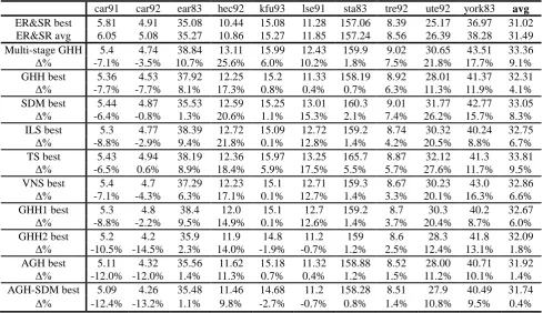
Table 2: Comparison results of ER&SR with various GHH related algorithms (Δ% denotes the relative percentage deviation for the value on the above row from the “ER&SR best”)
car91 car92 ear83 hec92 kfu93 lse91 sta83 tre92 ute92 york83 avg ER&SR best 5.81 4.91 35.08 10.44 15.08 11.28 157.06 8.39 25.17 36.97 31.02 ER&SR avg 6.05 5.08 35.27 10.86 15.27 11.85 157.24 8.56 26.39 38.28 31.49 Multi-stage GHH 5.4 4.74 38.84 13.11 15.99 12.43 159.9 9.02 30.65 43.51 33.36 Δ% -7.1% -3.5% 10.7% 25.6% 6.0% 10.2% 1.8% 7.5% 21.8% 17.7% 9.1% GHH best 5.36 4.53 37.92 12.25 15.2 11.33 158.19 8.92 28.01 41.37 32.31
Δ% -7.7% -7.7% 8.1% 17.3% 0.8% 0.4% 0.7% 6.3% 11.3% 11.9% 4.1%
SDM best 5.44 4.87 35.53 12.59 15.25 13.01 160.3 9.01 31.77 42.77 33.05 Δ% -6.4% -0.8% 1.3% 20.6% 1.1% 15.3% 2.1% 7.4% 26.2% 15.7% 8.3% ILS best 5.3 4.77 38.39 12.72 15.09 12.72 159.2 8.74 30.32 40.24 32.75
Δ% -8.8% -2.9% 9.4% 21.8% 0.1% 12.8% 1.4% 4.2% 20.5% 8.8% 6.7%
TS best 5.43 4.94 38.19 12.36 15.97 13.25 165.7 8.87 32.12 41.3 33.81
Δ% -6.5% 0.6% 8.9% 18.4% 5.9% 17.5% 5.5% 5.7% 27.6% 11.7% 9.5%
VNS best 5.4 4.7 37.29 12.23 15.1 12.71 159.3 8.67 30.23 43.0 32.86
Δ% -7.1% -4.3% 6.3% 17.1% 0.1% 12.7% 1.4% 3.3% 20.1% 16.3% 6.6%
GHH1 best 5.3 4.8 38.4 12.0 15.1 12.7 159.2 8.7 30.3 40.2 32.67
Δ% -8.8% -2.2% 9.5% 14.9% 0.1% 12.6% 1.4% 3.7% 20.4% 8.7% 6.0%
GHH2 best 5.2 4.2 35.9 11.9 14.8 11.2 159 8.6 28.3 41.8 32.09
Δ% -10.5% -14.5% 2.3% 14.0% -1.9% -0.7% 1.2% 2.5% 12.4% 13.1% 1.8% AGH best 5.11 4.32 35.56 11.62 15.18 11.32 158.88 8.52 28.00 40.71 31.92
Δ% -12.0% -12.0% 1.4% 11.3% 0.7% 0.4% 1.2% 1.5% 11.2% 10.1% 1.4% AGH-SDM best 5.09 4.26 35.48 11.46 14.68 11.2 158.28 8.51 27.9 40.49 31.74
Δ% -12.4% -13.2% 1.1% 9.8% -2.7% -0.7% 0.8% 1.4% 10.8% 9.5% 0.4%
1. Table 2 then gives the comparison results of our ER&SR algorithm with a number of Graph-based Hyper-Heuristic (GHH) algorithms which also use the same four graph-based heuristics (i.e. largest degree first, largest weighted Hyper-Heuristic (GHH): Tabu search is employed to search for the list of low level heuristics (Burke et al. 2007).
2. Steepest Descent Method (SDM): The best heuristic sequence among neighbourhoods is always selected if it is better than or the same as the current one (Qu and Burke 2009).
3. Iterated Local Search (ILS): The search is re-started after a certain number of iterations of SDM (Qu and Burke 2009).
4. Tabu Search (TS): The TS employed here is similar to that of GHH. The difference is that no greedy local search is further carried out on the complete solutions at each step (Qu and Burke 2009).
5. Variable Neighbourhood Search (VNS): The VNS employed is an iterative process where search is re-started after a certain number of walks are made by a standard VNS (Qu and Burke 2009).
7. Local Improvement during the Solution Construction (GHH2): During the solution construction by a heuristic sequence, at each step, the 1st event in the ordered list is scheduled into the partial solution, upon which a greedy search is implemented (Qu and Burke 2009).
8. Adaptive GHH (AGH): It is similar to the GHH, but focusing on developing an adaptive approach where heuristics are dynamically hybridised during solution construction (Qu et al. 2009).
9. AGH-SDM: An AGH, following by the steepest descent method to make improvement (Qu et al, 2009).
Table 2 shows that the ER&SR’s results are generally better than any of the previous proposed GHH related algorithms. In terms of the absolute objective function value, the ER&SR’s average result for the 10 test instances is 31.02, while the results of the other algorithms are ranged from 31.74 (for the AGH-SDM) to 33.81 (for the TS). In terms of the relative percentage deviation, the difference is more obvious: the ER&SR’s result is 0.4% better than the AGH-SDM and 9.5% better than the TS. The times to obtain our results are ranged from less than 1 minute for small instances (e.g. Sta83) to several hours for large instances (e.g. car91 and car92), which are at the same levels of those GHH related algorithms.
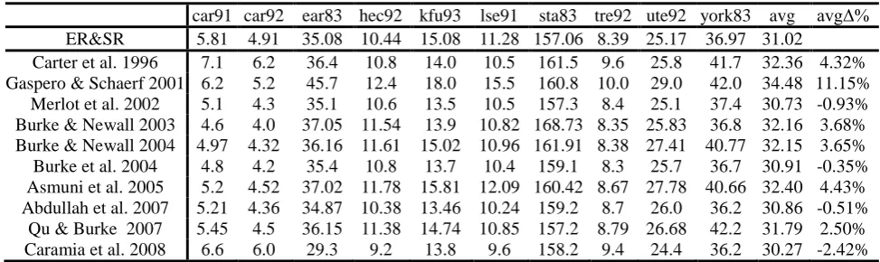
[image:11.595.53.540.386.531.2]To gain a better insight of the ES&SR’s performance, Table 3 lists the results of the state-of-the-art approaches which include a selection of appropriate methods that generate the best results among all of the approaches in the literature. These algorithms do not use any of the four graph based heuristics as the low level heuristics for solution construction. They generally use another class of techniques which implement local search (such as swaps and moves) to achieve improvement from an refined initial solutions. Since the solution disruption is restricted to just one or two units, these algorithms are very quick to generate each single new solution, but in theory they should be generally easy to get stuck in local optima.
Table 3: Comparison with results of non-GHH related algorithms in the literature (Δ% denotes the relative percentage deviation from the “ER&SR”)
car91 car92 ear83 hec92 kfu93 lse91 sta83 tre92 ute92 york83 avg avgΔ% ER&SR 5.81 4.91 35.08 10.44 15.08 11.28 157.06 8.39 25.17 36.97 31.02
Carter et al. 1996 7.1 6.2 36.4 10.8 14.0 10.5 161.5 9.6 25.8 41.7 32.36 4.32% Gaspero & Schaerf 2001 6.2 5.2 45.7 12.4 18.0 15.5 160.8 10.0 29.0 42.0 34.48 11.15%
Merlot et al. 2002 5.1 4.3 35.1 10.6 13.5 10.5 157.3 8.4 25.1 37.4 30.73 -0.93% Burke & Newall 2003 4.6 4.0 37.05 11.54 13.9 10.82 168.73 8.35 25.83 36.8 32.16 3.68% Burke & Newall 2004 4.97 4.32 36.16 11.61 15.02 10.96 161.91 8.38 27.41 40.77 32.15 3.65% Burke et al. 2004 4.8 4.2 35.4 10.8 13.7 10.4 159.1 8.3 25.7 36.7 30.91 -0.35% Asmuni et al. 2005 5.2 4.52 37.02 11.78 15.81 12.09 160.42 8.67 27.78 40.66 32.40 4.43% Abdullah et al. 2007 5.21 4.36 34.87 10.38 13.46 10.24 159.2 8.7 26.0 36.2 30.86 -0.51%
Qu & Burke 2007 5.45 4.5 36.15 11.38 14.74 10.85 157.2 8.79 26.68 42.2 31.79 2.50% Caramia et al. 2008 6.6 6.0 29.3 9.2 13.8 9.6 158.2 9.4 24.4 36.2 30.27 -2.42%
One may observe from Tables 2 and 3 that, at least for the exam timetabling problems, results by the class of hyper-heuristic (i.e. GHH relative algorithms) which use a set of graph based heuristics for solution construction are generally worse than those by the class of local search algorithms. This is not a surprise due to the computational complexity that these low level heuristics cause (Li et al. 2011). Let m be the number of exams, n be the number of available timeslots, and α be the graph density of the problem. Both Heuristics H1
(largest degree first) and H2 (largest weighted degree first) have computational complexity of O(m 2
n) to construct a complete solution, For heuristic H3 (largest color degree first), its complexity is O(αm
3
+m2n). For heuristic H4 (least saturation degree first), empirical studies have shown that it performs the best among all
the graph based heuristics. However, as a cost its complexity is as high as O(αm3n+m2n) which means constructing a solution by this heuristic is likely thousands times slower than a simple swap/move heuristic used for local search.
ER&SR, the difference are 0.93%, 0.35% and 0.51%, respectively. Compared to the algorithm presented in (Caramia et al. 2008), the ER&SR underperforms by 2.5% on average result but still outperforms on 4 of the 10 test instances. The above results support our motivation of developing the ER&SR, which is indeed something flexibly standing in between the constructive search and local search, although more sophisticated design and parameter setting at each step of its implementation are still required to maximise its performance for real world problems.
5 Conclusion
In this paper, we present a new approach based on the original idea of R&R, by incorporating two additional operators of Selection and Mutation in its Evolutionary Ruin step. In our proposed ER&SR, a cycle of Solution Decomposition, Evolutionary Ruin, Stochastic Recreate and Solution Acceptance is executed until a pre-defined stopping condition is reached. Taken as a whole, the ER&SR implements evolution within a single solution and carries out iterative search by component evaluation, solution disruption and stochastic rebuild. Experimental results on 10 exam timetabling benchmark problems have demonstrated the strength of the proposed approach.
We also propose a state transition based formal framework for a simplified version of the ER&SR, in which Stochastic Recreate restricts to probabilistic moves among different possible destination states based on the objective function values of the neighbouring solutions. We focus on the study of the ER&SR’s convergence behaviour by a finite Markov chain analysis. Our main result is that although the ER&SR algorithm can reach the global optimum after finite number of transitions with probability one, the algorithm does not converge to the global optimum. Of course, like other algorithms (such as genetic algorithm) which simply keep the best solution found over time, the ER&SR may converge to the global optimum geometrically fast. In addition, we study the ER&SR’s property on the stationary probability distribution on individual states: it is not only affected but also controllable by a proper combination of the Selection function, the Mutation rate and the Stochastic Recreate method. The last result suggests that, if properly implementing the ER&SR algorithm, the optimal solution of the problem still may have a stationary probability close to one even if we don’t use the strategy of reserving the best solution.
The SE&RE approach may be regarded as a general framework, in which many well-known search methods belong to its special case. For example, assume at each iteration x components are removed from an n -component solution, and let p be the acceptance criterion.
10. If x = 0, then it is a non-iterative method as only one single solution will be generated; 11. If x ≤ 3, then it is a local search method that uses small moves to change the configurations; 12. If x = n, then it is a constructive method with random starting points;
13. If (no Solution Decomposition) & (no Selection), then it equals to the R&R principle;
14. If (no Selection) & (no Mutation) & (Stochastic Recreate at specific orders), then it equals to the squeaky heel optimisation.
With regard to improvements on algorithmic design, the architecture of the ER&SR is innovative, and thus there is still some room for further improvement. In the Solution Decomposition part, we will study the formulation of domain knowledge for different types of other problems and the influence of different evaluation rules. In the Evolutionary Ruin part, we will study the suitable range for the number of components to be destroyed and the condition of applying a large move or a small move. For the Stochastic Recreate part, we will study the types of reconstruction methods that are unsuited for generating optimum or near-optimum results. Furthermore, we will evaluate the proposed algorithm with different operators applied in its three parts and the best combination we should try.
Acknowledgment
The work was supported by Ningbo Natural Science Foundation (under grand 2012A610026) and Natural Science Foundation of China (under grants 70971044 and 71171087).
References
S. Abdullah, S. Ahmadi, E.K. Burke; and M. Dror. 2007. “Investigating Ahuja-Orlin's Large Neighbourhood Search for Examination Timetabling.” OR Spectrum 29, 351-372.
U. Aickelin U., E.K. Burke E.K. and Li J. 2009. “An Evolutionary Squeaky Wheel Optimisation Approach for Personnel Scheduling”, IEEE Transactions on Evolutionary Computation 13(2): 433-443.
H. Asmuni, E.K. Burke, and J. Garibaldi. 2005. “Fuzzy Multiple Ordering Criteria for Examination Timetabling.” Practice and Theory of Automated Timetabling. Springer Lecture Notes in Computer Science 3616, 334-353.
E.K. Burke, Y. Bykov, J.P. Newall, and S. Petrovic. 200. “A Time-Predefined Local Search Approach to Exam Timetabling Problems.” IIE Transactions 36, 509-528.
E.K. Burke, T. Curtois, M. Hyde, G. Kendall, G. Ochoa, S. Petrovic, and J.A. Vazquez-Rodriguez. 2009. “HyFlex: A Flexible Framework for the Design and Analysis of Hyper-heuristics.” In Proceedings of Multidisciplinary International Scheduling Conference (MISTA 2009).
E.K. Burke, G. Kendall, and E. Soubeiga. 2003. “A Tabu-search Hyperheuristic for Timetabling and Rostering.” Journal of Heuristics 9, 451-470.
E.K. Burke, B. McCollum, A. Meisel, S. Petrovic; and R. Qu. 2007. “A Graph-based Hyper-heuristic for Educational Timetabling Problems.” European Journal of Operational Research 176, 177-192.
E.K. Burke and J.P. Newall. 2003. “Enhancing Timetable Solutions with Local Search Methods.” Practice and Theory of Automated Timetabling. Springer Lecture Notes in Computer Science 2740, 195-206. E. K. Burke and J.P. Newall. 2004. “Solving Examination Timetabling Problems through Adaptation of
Heuristic Orderings.” Annals of operations Research 129: 107-134.
E.K. Burke, S. Petrovic, and R. Qu. 2006. “Case Based Heuristic Selection for Timetabling Problems,” Journal of Scheduling 9, 115-132.
M. Carter, G. Laporte, and S. Lee. 1996. “Examination Timetabling: Algorithmic Strategies and Applications.” Journal of Operations Research Society 47, 373-383.
M. Caramia, P. DellOlmo, and G. Italiano. 2001. “New Algorithms for Examination Timetabling.” Algorithm Engineering. Springer Lecture Notes in Computer Science 1982, 230-241.
S. Casey and J. Thompson. 2004. “GRASPing the Examination Scheduling Problem.” Practice and Theory of Automated Timetabling. Springer Lecture Notes in Computer Science 2740, 232-244.
B. Cheang, H. Li, A. Lim, and B. Rodrigues. 2003. “Nurse Rostering Problems: a Bibliographic Survey.” European Journal of Operational Research 151, 447-460.
L.D. Gaspero and A. Schaerf. 2001. “Tabu Search Techniques for Examination Timetabling.” Practice and Theory of Automated Timetabling. Springer Lecture Notes in Computer Science 2079, 104-117.
G. Dueck and T. Scheuer. 1990. “Threshold Accepting: a General Purpose Optimization Algorithm Appearing Superior to Simulated Annealing.” Journal of Computational Physics 90, 161-175.
K. Dowsland and J. Thompson. 2005. “Ant Colony Optimization for the Examination Scheduling Problem." Journal of Operations Research Society 56, 426-438.
K. Easton, G. Nemhauser, and M. Trick. 2004. “Sports Scheduling.” In Handbook of Scheduling: Algorithms, Models, and Performance Analysis, J. Leung (ed.). Chapter 52, CRC Press.
W. Erben 2001. “A Grouping Genetic Algorithm for Graph Colouring and Exam Timetabling.” Practice and Theory of Automated Timetabling. Springer Lecture Notes in Computer Science 2079, 132-156.
C.H. Häll and A. Peterson. 2013. “Improving Paratransit Scheduling using Ruin and Recreate Methods.” Transportation Planning and Technology 36(4), 377-393.
P. Hansen and N. Mladenović. 1999. “Variable Neighbourhood Search: Principles and Applications.” European Journal of Operational Research 130, 449-467.
R.M. Karp 1983. “Reducibility Among Combinatorial Problems.” Complexity of Computer Computations 4, 85-103.
L.B. Koralov and Y.G. Sinai, Theory of Probability and Random Processes, Springer, 2007.
R.S.K. Kwan. 2004. “Bus and Train Driver Scheduling.” Handbook of scheduling: Algorithms, Models, and Performance Analysis, Chapter 51. CRC Press.
J. Li, E.K. Burke and R. Qu. 2011. “Integrating Neural Network and Logistic Regression to Underpin Hyper-heuristic Search.” Knowledge-Based Systems 24(2), 322-330.
J. Li, E.K. Burke, T. Curtois, S. Petrovic, and R. Qu. 2012a. “The Falling Tide Algorithm: a New Multi-objective Approach for Complex Workforce Scheduling.” OMEGA – The International Journal of Management Science 40, 283-293.
J. Li, R. Qu, and Y. Shen. 2012b. “Evolutionary Ruin and Stochastic Recreate: a Case Study on the Exam Timetabling Problem”, in Proceedings of the 26th European Conference on Modelling and Simulation (ECMA2012), pp. 347-353.
A. Misevicius. 2003a. “Genetic Algorithm Hybridized with Ruin and Recreate Procedure: Application to the Quadratic Assignment Problem.” Knowledge-Based Systems 16: 261-268.
A. Misevicius. 2003b. “Ruin and Recreate Principle Based Approach for the Quadratic Assignment Problem.” In Proceedings of Genetic and Evolutionary Conference (GECCO 2003). Springer Lecture Notes in Computer Science 2723, 598-609.
L. Merlot, N. Boland, B. Hughes, and P. Stuckey. 2002. “A Hybrid Algorithm for the Examination Timetabling Problem.” Practice and Theory of Automated Timetabling. Springer Lecture Notes in Computer Science 2740, 207-231.
L. Paquete and C.M. Fonseca. 2001. “A Study of Examination Timetabling with Multiobjective Evolutionary Algorithm.” In Proceedings of the 4th Meta-heuristics International Conference (MIC 2001), 149-154. S. Petrovic and E.K. Burke. 2004. “University Timetabling.” Handbook of Scheduling: Algorithms, Models,
and Performance Analysis. Chapter 45, CRC Press.
R. Qu and E.K. Burke. 2009. “Hybridizations Within a Graph based Hyper-heuristic Framework for University Timetabling Problems.” Journal of the Operational Research Society 60, 1273-1285.
R. Qu, E.K. Burke, and B.McCollum. 2009. “Adaptive Automated Construction of Hybrid Heuristics for Exam Timetabling and Graph Colouring Problems.” European Journal of Operational Research 198(2): 392-404.
R. Qu, E.K. Burke, B. McCollum, L.T.G. Merlot, and S.Y Lee. 2009. “A Survey of Search Methodologies and Automated System Development for Examination Timetabling.” Journal of Scheduling12, 5-89. A. Schaerf 1999. “A Survey of Automated Timetabling.” Artificial Intelligence Review 13, 87-127.
G. Schrimpf, J. Schneider, H. Stamm-Wilbrand, and G. Dueck. 2000. “Record Breaking Optimization Results using the Ruin and Recreate Principle.” Journal of Computational Physics 159, 139-171.
J. Thompson and K. Dowsland, 1998. “A Robust Simulated Annealing based Examination Timetabling System.” Computer & Operations Research 25, 637-648.
H.C. Tijms, A First Course in Stochastic Models. John Wiley & Sons Ltd, 2003.