ISSN 0962-4031
UNIVERSITY OF ST. ANDREWS
A Salience Theory of Choice Errors
Paola Manzini and Marco Mariotti
No.
1003
DISCUSSION PAPER SERIES
SCHOOL OF ECONOMICS & FINANCE
St. Salvator's College
St. Andrews, Fife KY16 9AL
A Salience Theory of Choice Errors
Paola Manzini
Marco Mariotti
yApril 2010
Abstract
We study a psychologically based foundation for choice errors. The decision
maker applies a preference ranking after forming a ‘consideration set’prior to choos-ing an alternative. Membership of the consideration set is determined both by the
alternative speci…csalience and by the rationality of the agent (his general propen-sity to consider all alternatives). The model turns out to include a logit formulation as a special case. In general, it has a rich set of implications both for exogenous
parameters and for a situation in which alternatives can a¤ect their own salience (salience games). Such implications are relevant to assess the link between ‘revealed’
preferences and ‘true’ preferences: for example, less rational agents may paradox-ically express their preference through choice more truthfully than more rational
agents.
J.E.L. codes: D0.
Keywords: Discrete choice, Random utility, Logit model, Consideration sets, bounded rationality
We thank Mauro Papi and Ivan Soraperra for helpful comments and discussions. Financial support from ESRC grant RES-000-22-3474 is gratefully acknowledged.
yBoth authors at School of Economics and Finance, University of St. Andrews, Castlecli¤e, The
1
Introduction
A vast class of models of choice assume deterministic behaviour. This holds both for the classical ‘rational’model (e.g. Samuelson [22], Richter [17]) and for more recent models of boundedly rational choice. But empirical economists have always had to confront the noisiness of the data. This raises the need to graft an appropriate error structure on the model, and therefore leads to the construction of a probabilistic choice model. Pioneering theoretical contributions in this area have been Luce [7] and Block and Marshak’s [2] and Marshak’s [15] Random Utility Maximization (RUM) model. In this paper we present a simple model of probabilistic choice from discrete choice sets (including RUM as a special case), with two main features:
1) The stochastic components of the model is given a precise interpretation.
2) Some parameters governing those components are endogenised via an equilibrium process.
The RUM model culminated in its most in‡uential version, McFadden’s ([10], [11])
conditional logit (or multinomial logit) discrete choice model, in which the probability
p(ai; A) that alternativeai is selected from a choice setA takes the form
p(ai; A) = exp (u(ai))=
X
aj2A
exp (u(aj)),
where u(aj) expresses the ‘systematic utility’ of alternative aj.1 This model is a case
within a general class in which alternativeai generates a ‘random utility stimulus’u(ai) +
"i, where"i is an error term, and is chosen over alternativeaj ifu(ai) u(aj)> "j "i. In
this perspective, the crucial step consists of de…ning an appropriate probabilistic structure on the errors. The logit model follows from the "i taking on i.i.d. Gumbel (or extreme
value type I) distributions2. A probit model would follow instead by assuming normal
distributions. In general, the basic constraint is that larger errors are made with smaller
1In applications, it is usually assumed further that utility is a linear function of the alternative
at-tributes.
probabilities, from which it follows that better alternatives are chosen with higher prob-ability. Closely related ideas have also found their way in modelling strategic behaviour, for the …rst time with McKelvey and Palfrey’s ([13], [14]) notion of Quantal Response Equilibrium (QRE)3.
This approach has proved to be extremely useful for experimental and empirical eco-nomics. But it seems fair to say that - beside the basic constraint of error monotonicity in utility - the error structure is not given a clear psychological foundation. Rather, it is chosen for analytical convenience from a standard set of statistical distributions, and then is added on to a determinsitic model. In other words, economic (or psychological) theory stops at the level of utility maximisation. ‘Bounded rationality’follows from exogeneous random errors. This makes the error structure rather di¢ cult to assess and interpret.4
We propose here a di¤erent route: we formulate directly a boundedly rational model of choice wihich includes some stochastic components. The main advantage of doing so is that the error structure becomes fully transparent, being part of the core model itself. The stochastic components of this model are extremely simple and, especially, can be given a precise psychological interpretation.
The model focusses on the notion of aconsideration set. The agent does not rationally evaluate all objectively available alternatives, but only a (possibly strict) subset of them, the consideration set. Once a consideration set has been formed, a choice is made by means of a preference relation, which in this paper we assume to be standard (complete and transitive). This two-step conceptualisation of the act of choice is rooted in psychology
3See Goeree, Holt and Palfrey [4] for an overview.
4In his Nobel lecture, McFadden [12] recounts of how he …rst developed the model in response to
a speci…c practical problem, and then sought a theoretical foundation, which he found in the Gumbel error speci…cation within RUM theory. We recall here that the Gumbel distribution function can be seen as the limit distribution function of (a suitable transformation of) the maximum value statistics for a sample of N i.i.d. random variables, as N tends to in…nity. The statistics needs to be appropriately transformed when taking the limit since, obviously, lettingG:be the common distribution function of the random variables and GM the distribution function of max (Xi)
i=1;:::;N, we have limN!1 GM(x) =
limN!1(G(x))N = 0for any xunlessG(x) = 1. Even this brief account of the error structure behind
and marketing science, but it has begun to di¤use in economics. Several recent models of boundedly rational choice adopt it in one way or the other (Manzini and Mariotti [8], Eliaz and Spiegler [3], Masatlioglu, Nakajima and Ozbay [9])5.
In our model the formation of the consideration set is stochastic. It is in fact the only stochastic component of the model. For an alternative, the probability of membership of the consideration set depends on two types of parameters (probabilities). The …rst parameter (‘rationality’), expresses the general propensity of the agent to consider all alternatives. The second parameter i (‘salience’) is alternative speci…c. We present two
natural models (called AND and OR) that depend on the speci…c way the parameters combine to determine the probability of membership of the consideration set.
We show that for a special case (that of equal salience across alternatives) both models can be expressed in a logit format. However, we use onlyordinal preference information. Contrast this with the logit model which uses, as explained above, equations of the type
u(ai) u(aj)> "j "i. These equations are only invariant to common cardinal (a¢ ne)
transformations of the u and the errors, andf therefore contain cardinal information. One advantage of expressing rationality in parametric form is that makes it easy to study how the probability of a given alternative being chosen varies with rationality. We …nd that some of the ‘intuitive’properties of error do not hold. One might expect, for example, that as rationality increases the agent will tend to choose each nonoptimal alternative with lower and lower probability: but we show that this is not necessarily the case. Both the AND and the OR models predict either monotonic or single peaked relationships between and the probability of choice, for all alternatives. The AND model predicts, for all alternatives and all parameters, an interval (and possibly the full interval) in which the probability of choice increases with rationality. The OR model predicts an increasing interval for some alternatives and some parameter con…gurations, but forbids increasingness on the whole range except for the best alternative. Unexpected e¤ects may also occur (in the OR model) in respect of the odds (probability ratio) of choosing a better alternative over a worse alternative, which may decrease with . And in both
5These three models are examples of the modern ‘sophisticated models of choice behavior which are
models the odds fail Luce’s [7] Independence of Irrelevant Alternatives test (which implies, together with other assumptions, the logit model)6. Salience enters these relationships in
a non-obvious way.
In the second part of the paper we endogenise salience. We consider situations in which alternatives can in‡uence their own salience. There are many examples that …t this case. In electoral contests, politicians make statements to get noticed by the voters, not only to persuade them. Voters may not consider certain parties for cultural reasons or out of habit7 (see Wilson [24] for a consideration set approach to political competition).
In animal mate competition the alternatives are male animals, the chooser is a female, and salience is controlled via natural selection (e.g. endowing peacocks with more or less showy tails), or by human activities (hair-styling, body-building, wealth-accumulation). In an I.O. context the alternatives are products, and salience is controlled via marketing strategies (Eliaz and Spiegler’s [3] work mentioned before is the …rst to study in detail this type of competitive situation).8
Our main result is that, when alternatives can fully control their own salience (‘ab-solute salience’), in equilibrium - under very general assumptions - both models have a ‘the showiest is the best’ feature: the equilibrium ordering of salience fully re‡ects the preference ordering over alternatives.
However, when salience is relative (so that alternatives can control salience only par-tially), there exists fully perverse equilibria in both models. In such equilibria the worst alternative has the highest probability of being chosen.
All these results have a bearing for the inferences we draw on true preferences us-ing revealed preferences reconstructed from choice data. We brie‡y comment on such
6In its core version. The nested logit, for example, allow for violations of IIA. A probit model also
allows for such violations. See e.g. Agresti [1] for an overview of statistical methods for categorical data.
7In Wilson [24], for example, it is reported that African Americans tend to ignore Republican
candi-dates in spite of the overlap betwen their policy preferences and the stance of the Republicans, and even if they are dissatis…ed with the Democratic candidate.
8Examples in our discipline of factors a¤ecting salience might be the choice of research topic, or the
implications in the concluding section.
2
Salience and rationality
2.1
The Model
There is a countable (possibly …nite) choice set of alternatives A = fa1; :::; an; :::g. The
agent has a strict preference ordering on A. We will often refer to the position of an alternative in the ranking as itsquality, with a loweriindicating a higher quality, so that
ai aj i¤i < j.
While a standard rational consumer explores the entire choice set A and picks the maximal element according to , here is applied only to aconsideration set C(A) A
of alternatives (the set of alternatives he actively considers). We allow for the consider-ation set to be empty, in which case the chooser picks a default option a (e.g. walking away from the shop, remaining without a partner, abstaining from voting).
Membership of C(A) for the alternatives in A is probabilistic. The probability of membership combines two components (probabilities): an idiosyncratic component i 2
[0;1] which is speci…c to the alternative and an alternative-independent component 2
(0;1). We call the probability i the salience of alternative ai, and a list( 1; :::; n; :::) a
salience pro…le. Note that while we use the term salience throughout for simplicity and because it tallies with leading examples, there are situations in which i is not associated
withawareness of the alternative by the agent, but rather with the resistance of the agent to consider the alternative for choice (e.g. for ideological reasons).
The probability measures the general propensity of the agent to consider all alter-natives. All else being equal, an agent with a higher is more likely, coeteris paribus, to apply his preference to the entire choice set A and can thus be interpreted as the agent’s degree of rationality.
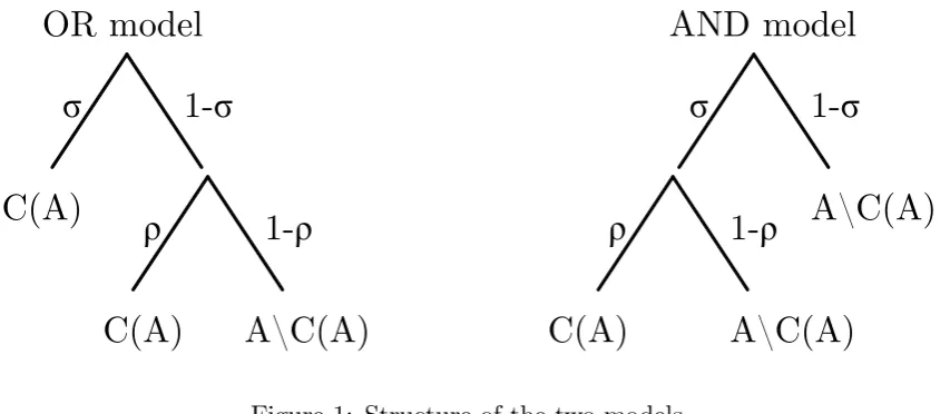
We consider two elementary probability models, both of which determineC(A)in two stages, as depicted in …gure 1. The sets at the terminal nodes indicate the destination of the alternative.
OR model
AND model
C(A)
A\C(A)
A\C(A)
C(A)
A\C(A)
C(A)
_
1-
_
_
1-
_
[image:8.595.89.516.72.258.2]a
1-
a
a
1-
a
Figure 1: Structure of the two models
then all alternatives which haven’t been drawn in this way are considered with probability . So
prob(ai 2C(A)) = i+ (1 i)
AND model: any alternative ai is provisionally drawn into the consideration set with
probability i, and it remains there with probability . So
prob(ai 2C(A)) = i
In both models, once the probabilistic consideration phase has been completed and a set C(A) has been formed, the agent chooses (if C(A) is nonempty) the alternative ai
with the properties that
ai 2C(A) and ai aj for all aj 2C(A)n faig
If C(A) is empty he chooses the default optiona .9
Finally, observe that the models are invariant to permuting the order in which salience and rationality are applied.
2.2
The Logit Retrouvé?
There is a formal relation between these models and the RUM models. We begin by discussing a benchmark situation, in which both models collapse to a logit form. Let
9The default option could be replaced by a more complex procedure to arrive at a choice, notably
pAN D(ai; A) and pOR(ai; A) denote the probabilities of choice conditional on the agent
picking an element inA in the AND and in the OR model, respectively.
Proposition 1 There exists a utility functionu:A !Rerepresenting onA, a salience pro…le, and coe¢ cients ; 0; ; 0 such that p
AN D(ai; A) and pOR(ai; A) can be written
in logit form, that is
pOR(ai; A) = exp ( + u(ai))=
X
j
exp ( + u(aj))
pAN D(ai; A) = exp ( 0+ 0u(ai))=
X
j
exp ( 0 + 0u(aj)),
To see this, let’s write down the choice probabilities explicitly. In the OR model, the probability pOR(ai) that ai 2A is chosen is10:
pOR(ai) = i
Y
j<i
((1 j) (1 ))
| {z }
+ (1 i)
Y
j<i
((1 j) (1 ))
| {z }
probability that ai entersC in the
…rst stage and the alternatives better than ai do not enter C
probability thatai enters C in the
second stage and the alternatives better than ai do not enter C
that is
pOR(ai) = ( i+ (1 i) ) (1 )i 1
Y
j<i
(1 j)
In the AND model, the probability pAN D(ai) that ai 2A is chosen is
pAN D(ai) = i
Y
j<i
(1 j)
| {z }
Y
j<i
(1 j)
| {z }
probability that ai enters C(A) in the
…rst stage and the alternatives better than ai do not enterC(A)
probability that ai remains in C(A) in
the second stage and the alternatives better than ai do not enter C(A)
that is,
pAN D(ai) = i
Y
j<i
(1 j)
10Use the convention thatQ0
Consider now the case of a common level of salience 2(0;1), with = i for alli. Then
the probability distributions are log-linear in quality
logpOR(ai) = (i 1)
logpAN D(ai) = 0 0(i 1),
with = log ( + ), = log (1 ) (1 ), 0 = log , and 0 = log (1 ).
It follows that, de…ning an (ordinal) utility functionurepresenting onAbyu(ai) = 1 i
we can write the probabilities of choice conditional on the agent picking an element inA
as in the statement of Proposition 1.
This observation provides a simple new psychological foundation for an often used error speci…cation. The OR and AND models can be seen in this perspective a class of ‘distortions’of the conditional logit model, where the distortions arise from di¤erences in salience between the alternatives. For example in the OR model
logpOR(ai) = log ( i+ (1 i) ) + (i 1) log (1 ) +
X
j<i
log (1 j)
and i may enter non-linearly in the expression through the termPj<ilog (1 j).
It is important, however, to bear in mind that the logit structure only holds for (a¢ ne transformations of) the particular utility speci…cation assumed. As our models useordinal
preference information as primitive, the probability of choice can only be invariant to that type of information. Some allowed utility transformations will destroy the loglinear relationships. In other words, at a fundamental level the log-linearity only holds with respect to the quality ranking index.
2.3
Limiting behavior
Curiously, the limiting version of the AND model for high rationality coincides with the limiting version of the OR model for low rationality,
lim
!1pAN D(a) = lim!0pOR(a) = i
Y
j<i
(1 j)
A moment’s re‡ection explains this with the fact that taking these opposit limits is the way to make consideration behavior be determined solely by salience in each of two models. Observe that the quality di¤erence e¤ect persists in the limit.
The limiting conditional probabilities of choice as vanishes are of interest:
lim
!0pOR(ai; A) = lim!0
( i + (1 i) ) (1 )i 1Qj<i(1 j)
X
k
( k+ (1 k) ) (1 ) k 1Q
j<k(1 j)
= i
1 + k
X
k<i
kQj<k (11
j)+
X
k>i
kQj<k(1 j)
and
lim
!0pAN D(ai; A) = lim!0
i
Q
j<i(1 j)
X
k
kQj<k(1 j)
= Xi
k k
These calculations highlight a further di¤erence from the logit (or quantal) models, which collapse to random choice as when the ‘rationality’parameter of the logit tends to
0. In general the limiting behaviour for that tends to0is not purely random choice in our models. In both the OR and the AND model the salience di¤erence between alternatives is preserved in the limit. In addition the quality di¤erence between alternatives is preserved in the limit in the OR model (though not in the AND model).
n).11 The OR model collapses instead to random choice in the limit of low rationality
provided that common salience also vanishes:
i = 2(0;1) for all i)
lim
!0lim!0pOR(ai; A) =
1
n
Note that the order matters in the above repeated limit.
2.4
Basic Comparative Statics Properties
Some comparative statics properties are immediate and, in both the OR and AND model, as expected:
(salience responsiveness)the probability of an alternative being chosen increases in the alternative’s own salience and decreases in the salience of the other alterna-tives;
(quality responsiveness) an increase in own quality12 increases the probability of the alternative being chosen;
(monotonicity) if the salience ranking is (weakly) the same as the inverse quality ranking (i.e. i < j ) i j), the probability that a better alternative is chosen is
higher than the probability that a worse alternative is chosen.13 However, the dis-tribution of salience may scramble this association between quality and probability of being chosen.
11Though not the OR model: in the common salience case we have
lim
!0pOR(ai; A)
=
2 1 X
k<i 1 (1 )i k
!
(1 )n i
12More precisely, a permutation of the objects in the preference order which improves the ranking of
the object.
13So in particular this holds for the case of equal salience
BecausepOR(ai)andpAN D(ai)areithdegree polynomials in , the e¤ect of an increase
in rationality is more subtle. In this respect the status of the best alternativea1 is di¤erent
from that of all the other alternatives. For a1 an increase in rationality is always good
news in both models, with
@pAN D(a1)
@ = (1 1)>0 @pOR(a1)
@ = 1 >0
(observe however that the two models have opposite implications concerning the e¤ect of salience on the impact of rationality).
A further observation stems from looking at the distribution functions, over quality levels, indicating the probability of choosing an alternative of at least a given level i of quality:
FOR(i) = 1 (1 )i
Y
j i
(1 j)
FAN D(i) = 1
Y
j i
(1 j)
from which it is evident that, in both models:
(cumulative rationality responsiveness) For any quality level i, the probabil-ity of choosing an alternative of qualprobabil-ity i or better is increasing in the degree of rationality.
But for individual alternatives di¤erent from the best, the probability of being chosen as a function of rationality depends in a non-obvious way on the parameters of the model.
3
Who gains from rationality?
3.1
OR model
In this section we discuss how the probability of choice for an alternative can vary non-monotonically (but with at most one peak) in the OR model as rationality increases.
@pOR(ai)
@ =
"
(1 i) (1 )
i 1Y
j<i
(1 j)
#
+
"
( i+ (1 i) ) (i 1) (1 ) i 2Y
j<i
(1 j)
#
= (1 )i 2(1 i i i(1 i) )
Y
j<i
(1 j)
which is ambiguous in sign. The decomposition highlights the source of ambiguity. On the one hand, an increase in increases the probability that ai will be considered by
the decision maker in the event, with probability (1 i), that it has not entered the
consideration set because of its salience; on the other hand, it also increases the probability that better alternatives are considered.
De…ning
1 i i
(1 i)i
we have
@pOR(ai)
@ >0, <
The threshold ranges in ( 1;1] and attains its maximum settingi = 1. Therefore
@pOR(ai)
@ is single peaked or monotonic on (0;1) and pOR(ai) attains a maximum, as a
function of 2 (0;1), at whenever 2 (0;1). For pOR(ai) to peak at positive levels
of , it must be that i < 1
i for otherwise 0. Quality and salience are substitutes to
maintain a given .
The set of alternatives can thus be partitioned into in three types (according to when an increase in rationality is good news for the alternative), which we record as:
Proposition 2 pOR(ai) has at most one peak as a function of 2 (0;1). It is always
increasing for i = 1. For any i > 1, pOR(ai) is strictly increasing on an initial range i¤
i i <1, and for su¢ ciently high, pOR(ai) is strictly decreasing.
- the top alternative, always;
- alternatives displaying a combination of good quality and low salience, at su¢ ciently low rationality levels.
An agent with higher rationality may be less attracted by a good alternative (but not the best) if it has high salience.
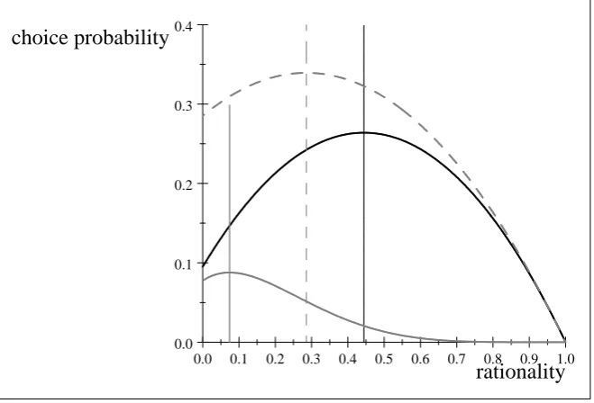
Note that only own salience, and not the salience of the other alternatives, a¤ects the value of and thus the sign of the derivative. The e¤ect of own salience on (namelyi i2) is negative fori >1and zero fori= 1. A lower quality (increase ini) reduces the threshold . The quality e¤ect and the salience e¤ect, as well as examples of choice probabilities peaking at intermediate degrees of rationality fo second (or worse) rate alternatives, are visualised in …gure 2. Here, with respect to a baseline case (black line, i = 2, i = 0:1)
quality is decreased (to i = 6) in the pOR(ai) represented by the gray solid line while
salience is increased (to i = 0:3) in the pOR(ai) represented by the grey dashed line.
0.0 0.1 0.2 0.3 0.4 0.5 0.6 0.7 0.8 0.9 1.0 0.0
0.1 0.2 0.3 0.4
[image:15.595.136.466.358.582.2]rationality choice probability
Figure 2: Comparative statics in the OR model: increasing i shiftspOR(ai)upwards and
3.2
AND model
The response of the probability of choice in the AND model as rationality increases is qualitatively di¤erent from that of the OR model, as we now demonstrate.
In order to highlight the role of it is instructive to rewrite the model with the following notation. Let S(m; k) denote the ordered set of combinations of k elements from the set f 1; :::; mg, where jS(m; k)j = mk , with all of the elements in S(m; k)
listed in ascending order lexicographically. Finally, let sm;k = 1;2; :::; mk denote the
corresponding index set and let S(m; k) (i) denote the i th element of S(m; k).
To see why this notation is useful, let for example i= 4 and compute the probability
pAN D(a4) that alternative a2 is selected. This is given by
pAN D(a4) = 4 ((1 1 ) (1 2 ) (1 3 ))
= 4 (1 1 2 3 + 2 3 2 + 1 2 2+ 1 3 2 1 2 3 3)
= 4 (1 ( 1+ 2+ 3) + 2( 1 2+ 1 3+ 2 3) 3 1 2 3)
The relevant index sets are s3;1 = f1;2;3g, s3;2 = f1;2;3g and s3;3 = f1g, so that
e.g. S(3;2) (1) = 1 2, S(3;2) (2) = 1 3, S(3;2) (3) = 1 3, and so on. Then we can
rewritepAN D(a4) as
pAN D(a4) = 4
0 @1 +
3
X
j=1
0
@( )j X
k2s3;j
S(3; j) (k)
1 A
1 A
In general, de…ning
A(i; j) = X
k2si 1;j
S(i 1; j) (k),
the probability that ai is chosen can be rewritten as:
pAN D(ai) = i 1 + i 1
X
j=1
( )jA(i; j)
!
We can now check how this varies with rationality:
@pAN D(ai)
@ = i 1 +
i 1
X
j=1
( )jA(i; j)
!
+ i
i 1
X
j=1
j( 1)j j 1A(i; j)
!
which yields
@pAN D(ai)
@ = i 1 +
i 1
X
j=1
(j+ 1) ( )jA(i; j)
Like in the OR model, the e¤ect of a change in on the probability of choice is ambiguous, but here there clearly exists b2 (0;1) such that @pAN D(ai)
@ > 0 if <b. But
unlike in the OR model, there cannot be any sure-…re loser from an increase in rationality: every alternative gains from increases in rationality, whatever the salience pro…le and the quality of the alternative, at su¢ ciently low levels of rationality (by taking away choice probability from the default alternativea ).
We now show that the threshold b, when it exists in (0;1), is unique.
Proposition 3 For all i, pAN D(ai)has at most one peak as a function of 2(0;1), and
it is strictly increasing on an initial range. Moreover pAN D(ai) can be strictly increasing
on the entire interval (0;1) even for i >1.
All (easy but mostly tedious) missing proofs are relegated to a separate section. The latter part of the statement highlights a major di¤erence from the OR model: in the AND model increases in rationality can be good news for inferior alternatives at all
levels of rationality, something which cannot happen in the OR model.
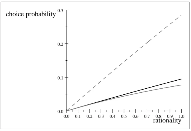
Note …nally that, unlike in the OR model, the entire salience pro…le is relevant to determine the impact of rationality. We display the salience and quality e¤ect in the graph below, using the same values as for the OR model:
3.3
Choice Odds and Menu E¤ects
We have noted that the e¤ect of an increase in rationality on the probability of choice of any alternative which is not the best is ambiguous. But what about theodds of choosing a better quality alternative over a lower quality alternative? Even if the probability of choosing an inferior alternative increases with rationality, one may conjecture that it does so at a lower speed than superior alternatives, so that the odds of making a better choice increase. This conjecture is clearly true in the AND model. De…ning, fori < j,
oddsAN D(i; j)
pAN D(ai)
pAN D(aj)
= i
j
Qj 1
k=i(1 k)
we have immediately
@oddsAN D(i; j)
0.0 0.1 0.2 0.3 0.4 0.5 0.6 0.7 0.8 0.9 1.0 0.0
0.1 0.2 0.3
[image:18.595.132.467.69.298.2]rationality choice probability
Figure 3: Comparative statics in the AND model: increasing i shifts pOR(ai) upwards;
increasingishiftspOR(ai)downwards. With these parameter values is always increasing
over the (0;1) interval.
But the conjecture is false in the OR model, at low levels of rationality and low levels of salience of the inferior alternative, irrespective of the quality di¤erence between the two alternatives.
De…ne, with i < j,
oddsOR(i; j)
pOR(ai)
pOR(aj)
= ( i+ (1 i) )
( j + (1 j) ) (1 )
j iQj 1
k=i(1 k)
Then we have
Proposition 4 For all i; j with i < j, there exists 2 (0;1) and j 2 (0;1) such that,
for < and j < j, @odds@OR(i;j) <0.
Observe that both expressions for the odds violate Luce’s [7] classical IIA axiom, which states that the choice probability ratio for two alternativesai andaj is independent of the
other alternatives in the choice set A. In our models14, this holds true only for changes
in A which remove or delete alternatives each of which is either better or worse than
both ai and aj. Inserting, for example, an alternative al with ai al aj in the choice
set would change the terms (1 )j iQjk=1i(1 k) and
Qj 1
k=i(1 k) which appear
in oddsOR(i; j) and oddsAN D(i; j), respectively. The insertion of such an intermediate
alternative would make no di¤erence regarding the probability of choice of the better al-ternativeai, but would create a new event of probability( l+ (1 l) ) ( j+ (1 j) )
in the OR model and( l ) ( j )in the AND model (namely the probabilities thatanand
aj are both considered), in which the lower quality alternative is not chosen. As a
par-ticular implication of these observations, this means that oddsOR(i; j)and oddsAN D(i; j)
are weakly increasing with the size of the choice set.
The dependence of the odds on the other available alternatives is often a realistic fea-ture, which applied economist have sought to incorporate, for example, in the conditional logit model.15 The blue bus-red bus problem is the standard example. Suppose the agent
chooses with probabilities one third each the train (t), a red bus (r) or a blue bus (b) as a means of transport, so that the choice odds for any two alternatives are1. Nevertheless, if r is removed from the choice set, it is natural to expect that the odds of choosing b
overt become2, rather than staying at1 as required by IIA. In our model (once adapted to include ranking ties), the natural exaplanation for why the odds should change (that the agent ranks a blue bus and a red bus in the same way) immediately yields the odds change.
4
Salience games
4.1
Absolute salience: The showiest is the best
We now imagine that alternatives can choose, possibly at a cost, the salience they pos-sess. This is natural in several contexts. For example, a minor politician can make an outrageous statement to get noticed by the media and enter the voters’ consideration set, but he will likely incur a cost in terms of credibility. One can increase expenditure on hairdressing to get noticed by potential partners. And …rms, of course, have huge advertising budgets.
15By adding a nested structure to choice process (nested logit) or by allowing heteroscedasticity of the
We are mainly interested in the question of how the equilibrium salience order cor-relates with the quality order (and in how this is re‡ected in choice probabilities). The answer is not obvious a priori as incentives seem to run both ways. On the one hand the best alternative has a strong incentive to get noticed: it fears no competition. On the other hand, the only weapon the inferior alternatives have to have a chance to be chosen is to increase their probability of entering the consideration set.
In this section we assume that there is a …nite number of alternatives, and that the strategy set for alternative ai is a …nite subset S of the unit interval (below we illustrate
how other domains could be considered). The payo¤ to each alternative is the expected probability of being chosen minus a (possibly negative) cost associated with the chosen salience level. One interpretation of this function is that alternatives either vie for one single chooser who chooses one alternative, or care about ‘market share’with a continuum of identical choosers each of whom chooses one alternative. Formally, let e be a function
e:S !Re. The payo¤ to alternative i for a pure strategy pro…le 2Sn is
zi( i; i) = ( i+ (1 i) ) (1 )i 1
Y
j<i
(1 j) e( i)
for the OR model and
zi( i; i) = i
Y
j<i
(1 j) e( i)
for the AND model. We make no assumption on the function e. In particular, e can be increasing or decreasing. So e could be intepreted as e¤ort, when increasing salience is costly, or as elation, when increasing salience is pleasurable.
Proposition 5 In both the AND and the OR model there exists an equilibrium in pure
strategies.
The proof makes clear that this pure strategy existence result continues to hold when
S is a compact subset of [0;1] and e(:) is continuous, or possibly discontinuous but increasing. The next characterisation result holds even more generally, for any structure of S [0;1] and anye(:).
Proposition 6 (The showiest is the best) Suppose ai aj and let ( 1; :::; n) be a pure
strategy equilibrium. Then, for all , i > j both in the AND and in the OR model.
Note that lower quality alternatives do not have any intrinsic disadvantage, in terms of salience enhancing technology, with respect to higher quality alternatives. The reason why they produce less salience in equilibrium does not derive from lower levels of resources or lower unit costs of salience production (as might be the case in a signalling story): every alternative can choose from exactly the same set at exactly the same cost or bene…t.
4.2
Relative salience: the ugly duckling can get picked most
often
So far we have assumed that each alternative can select its own salience independently of the salience of the other alternative. In this sense salience was absolute. This is appropriate in some contexts, e.g. if repeated ads in favour of an alternative merely have the function of making the agent aware of the alternative (‘did you know that people who read book A also read book B?’; ‘have you considered using a scooter to go to work’?), with i representing either the probability that the agent is aware or the proportion
of aware agents within a population. In other contexts, however, alternatives can only control variables that a¤ect salience in a relative way. If everybody else dresses in green you will be salient by dressing in yellow, and viceversa. If all other candidates converge on a given political message, you will be salient by deviating from that message. We call this the case of relative salience.
We show that in this case the neat equilibrium ordering obtained in proposition 6 breaks down. As a consequence, it is even possible that, in equilibrium, the worst alter-native is selected with the highest probability.
Suppose now that each alternative ai selects a ‘position’vi 2 [0;1], and that own
salience is determined by the entire pro…le of the vi’s. In particular, we assume that an
alternative’s salience is conferred by its di¤erence, in terms of position, from the ‘average alternative’(excluding itself)
i = vi
P
j6=ivj
(n 1)
2
The alternatives aim as usual at maximising the probability of being chosen, where the probability is computed according to either the AND or te OR model.
Proposition 7 The AND model admits (for some n) a pure strategy Nash equilibrium
in which, for any , the worst alternative has the highest probability of being chosen.
Proposition 8 The OR model admits (for some n) a pure strategy Nash equilibrium in
which, for su¢ ciently small, the worst alternative has the highest probability of being
chosen. For su¢ ciently high (for any n) the best alternative is chosen with the highest
probability.
The di¤erence between these two results stems from the di¤erence between the AND the OR model we highlighted before: at degrees of rationality near one, the OR model -but not the AND model - approximates well the standard utility maximisation model.
5
Proofs
Proof of Proposition 3: De…ne as in the text
A(i; j) = X
k2si 1;j
S(i 1; j) (k)
We have already observed that pAN D(ai) is strictly increasing on the initial range of
de…nition. We study the sign of @pAN D(ai)
@ , which depends on the sign of the expression
1 +
i 1
X
j=1
(j + 1) ( )jA(i; j) (*)
= 2 12 +
i 1
X
j=1
(j+ 1) ( )j 2A(i; j)
!
We show that there exists a single valueb2(0;1)at which @pAN D(a4)
@ vanishes. Suppose
to the contrary that there were two such values b2(0;1)and bb2(0;1), say withb<bb. Then, using the LHS side expression in equation * and the de…nition ofband bb,
i 1
X
j=1
(j + 1) ( b)jA(i; j) = 1 =
i 1
X
j=1
On the other hand, using the RHS in equation * and the de…nition of band bb,
i 1
X
j=1
(j+ 1) ( b)j 2A(i; j) = 1 (b)2
and
i 1
X
j=1
(j + 1) bb
j 2
A(i; j) = 1
bb 2
Therefore
i 1
X
j=1
(j + 1) ( b)j 2A(i; j) <
i 1
X
j=1
(j+ 1) bb
j 2
A(i; j)
so that
(b)2
i 1
X
j=1
(j+ 1) ( b)j 2A(i; j) < bb 2
i 1
X
j=1
(j+ 1) bb j 2A(i; j)
,
i 1
X
j=1
(j+ 1) ( b)jA(i; j) <
i 1
X
j=1
(j+ 1) bb jA(i; j)
a contradiction. Therefore there is at most one value of 2 (0;1) at which @pAN D(ai)
@
vanishes, from which (since @pAN D(ai)
@ is a polynomial and is strictly increasing on the
initial range of de…nition) the …rst part of the statement follows. The plot in the text shows examples for which pAN D(ai) is strictly increasing on the whole interval (0;1):
as is evident from the formula for pAN D(ai), this can be obtained by setting values of
1; :::; i 1 su¢ ciently low (note thatA(i; j) approximates i when 1; :::; i 1 are close
to zero).
Proof of Proposition 4: Di¤erentiate logarithmically and rearrange to obtain
@logoddsOR(i; j)
@ =
(1 i)
( i+ (1 i) )
+ (j i)
(1 )
(1 j)
( j + (1 j) )
which is negative for and j small enough. Conclude by noting that oddsOR(i; j) is
a positive function so that sign@logoddsOR(i;j)
@ =sign
@oddsOR(i;j)
@ .
Proof of Proposition 5: Consider the OR model. At a pure strategy equilibrium, alternative a1 simply solves the one-person problem
max
Let 1 be the solution to this problem. Now suppose inductively that for each i < j
the game restricted to alternativesa1; :::aj 1 has a pure strategy equilbrium 1; :::; j 1 .
Then the game between alternatives a1; :::aj (of which 1; :::; j 1 are indi¤erent to the
choice of alternativej) has the pure strategy equilbrium 1; :::; j , where j is a solution to the problem
max
j2Sj
( j+ (1 j) ) (1 )j 1
Y
i<j
(1 i) e( j)
So for anyn the game has a pure strategy equilbrium. A similar logic applies to the AND model.
Proof of Proposition 6: Consider the OR model. By contradiction, suppose that
ai aj but i < j. We use a revealed preference argument. Because i is optimal for
alternative ai, it must provide a weakly higher expected payo¤ than j, that is:
( i+ (1 i) ) (1 ) i 1Y
k<i
(1 k) e( i)
( j+ (1 j) ) (1 )i 1
Y
k<i
(1 k) e( j)
or
(( i+ (1 i) ) ( j+ (1 j) )) (1 )i 1
Y
k<i
(1 k)
e( i) e( j)
Since i < j and <1, we have( i+ (1 i) ) ( j + (1 j) )<0. Furthermore,
sinceai aj and thusi < j, we have that(1 )i 1Qk<i(1 k)>(1 )j 1Qk<j(1 k).
Therefore the previous displayed equation implies
(( i+ (1 i) ) ( j+ (1 j) )) (1 )j 1
Y
k<j
(1 k)> e( i) e( j)
But then
( i+ (1 i) ) (1 ) j 1Y
k<j
(1 k) e( i)
> ( j + (1 j) ) (1 )j 1
Y
k<j
which means that alternative j would gain by deviating from j to i, a contradiction.
The same argument works for the AND model. If ai aj it must be
( i )
Y
k<i
(1 k) e( i) ( j )
Y
k<i
(1 k) e( j)
or
( i j)
Y
k<i
(1 k) e( i) e( j)
Therefore if it were i < j we would have
( i j)
Y
k<j
(1 k)> e( i) e( j)
which contradicts the optimality of j foraj.
Proof of Proposition 7: We consider the case of three alternatives and claim that the position pro…le v = (0;0;1) is a Nash Equilibrium. For a generic pro…le v, the choice probabilities are given by
pAN D(a1; v) = v1 v2+2v3 2
pAN D(a2; v) = v2 v1+2v3 2
1 v1 v2+2v3 2
pAN D(a3; v) = v3 v1+2v2 2
1 v1 v2+2v3 2
1 v2 v1+2v3 2
It is seen immediately that alternative 1’s best replies to v2 = 0 and v3 = 1 are v1 = 1
and v1 = 0, so that it cannot pro…tably deviate from v . Turning now to alternative 2,
check
@pAN D(a2; v) @v2 v1=0
v3=1
= 1
8 (2v2 1) 8 5 v2 4 v
2 2
Studying the sign, it is straightforward to verify that the possible maxima are at v2 = 0
and, depending on the size of , either v2 = 12 or v2 = 1. The corresponding choice
probabilities are:
pAN D(a2; v ) =
1
4 1
1 4
pAN D a2; 0;
1
2;1 = 0
pAN D(a2;(0;1;1)) =
1
so that, regardless of the size of , alternative 2cannot pro…tably deviate from v . Finally consider alternative 3:
@pAN D(a3; v)
@v3 v1=0
v2=0
= 1
8 v3 v
2
3 4 3 v 2 3 4
The roots of the polynomial arev3 = 0,v3 = p2 andv3 = p23 , so that forv3 2[0;1]we
have that @pAN D(a3;v)
@v3 v1=0
v2=0
>0forv3 2 0;p23 andv3 > p2 , while @pAN D@v(3a3;v) v
1=0
v2=0
<0for
v3 2 p23 ;p2 . It follows that pAN D(a3;(0;0; v3))is maximised for v3 = min
n
1;p2
3
o
=
1. The corresponding choice probability is
pAN D(a3; v ) =
1
16 ( 4)
2
It is now straightforward to verify that
pAN D(a3; v )> pAN D(a1; v )> pAN D(a2; v )
Proof of Proposition 8: Consider again the case with three alternatives. The choice probabilities are now:
pOR(a1; v) = v1
v2+v3
2
2
+ 1 v1
v2+v3
2
2!
pOR(a2; v) =
= v2
v1+v3
2
2
+ 1 v2
v1+v3
2
2! !
1 v1
v2+v3
2
2!
(1 )
pOR(a3; v) =
= v3
v1+v2
2
2
+ 1 v3
v1+v2
2
2!!
1 v1
v2+v3
2
2!
1 v2
v1+v3
2
2!
Evaluating at v = (0;0;1) yields:
pOR(a1; v ) =
1
4(1 + 3 )
pOR(a2; v ) =
3
4(1 )
1
4(1 + 3 )
pOR(a3; v ) =
9
16(1 )
2
It is imediately apparent that pOR(a1; v ) > pOR(a2; v ). Moreover, for 2 (0;1), pOR(a3; v ) > pOR(a1; v ) if and only if < 5 2
p
5 3 <
1
3; and pOR(a3; v )> pOR(a2; v ) if
and only if < 13.
To verify thatv is an equilibrium, it is immediately checked that alternative1cannot pro…tably deviate from v . Turning now to alternative2;compute:
@pOR(a2; v) @v2 v1=0
v3=1
= 1
8( 1) 10 (1 )v
3
2 3 (1 )v 2
2+ 2 (7 11 )v2 (3 + 5)
Assume now that < 13. This implies that pOR(a2;(0; v2;1)) can only be maximised at v2 = 0 orv2 = 1. The corresponding choice probabilities are
pAN D(a2;(0;0;1)) =
3
16(1 + 3 ) (1 )
pAN D(a2;(0;1;1)) = 0
so that v2 = 0 is the best reply.
Turning …nally to alternative 3:
@pOR(a3; v) @v3 v1=0
v2=0
= 1
4v3(v3 2) (v3+ 2) (1 )
2
and it is easy to check that pOR(a2;(0;0; v3))is maximised in v3 = 0.
The second part of the statement follows trivially from inspection of the payo¤ func-tions.
6
Concluding remarks and related literature
utility maximisation. Admittedly, we have opened just one box. Other explanations, beside consideration sets, may be relevant. Recently Rubinstein and Salant [21] have studied an agent who expresses di¤erent preferences under di¤erent frames of choice. The link with this paper is that the set of such preferences is interpreted as a set of deviations from a true (welfare relevant) preference. However, their analysis takes a very di¤erent direction from ours in that it eschews any stochastic element. The probability model is, on the contrary, at the core of our theory.
There are also di¤erent plausible ways to model consideration sets and the compe-tition for them. The already mentioned work by Eliaz and Spiegler [3] studies in great detail the competition between two …rms, who choose marketing strategies to make their products enter the consideration sets of a continuum of identical consumers. The choice model at the heart of this work is an application of Masatlioglu, Nakajima and Ozbay [9], which is deterministic. Eliaz and Spiegler [3] also perform comparative statics exercises that relate to changes in rationality. One the main …ndings is that in some equilibria …rms do not increase their pro…ts compared to a situation in which consumers are fully rational (informed). More comparisons are made either by introducing in the population of boundedly rational consumers some rational consumers, or by changing the ‘consider-ation function’ (the function that determines the consider‘consider-ation set of consumers). One implication is that industry pro…ts are a non-monotonic function of changes in rationality thus de…ned.
A …rst general message from our paper is that ‘revealed preferences’are not necessarily a better guide to discovering true preferences when the rationality of the agent is higher (namely when the agent has a higher probability of being better informed about the available alternatives). For example, suppose you can observe or infer the degrees of rationality, and 0, under which two sets choices were made. Suppose that alternative
x is chosen more frequently over alternativeyin condition than in condition 0: it does
not necessarily follow from the fact that > 0 that x is more likely to be better that
y. Less rational agents (or agents choosing under worse informational conditions) may express their preference through choice more truthfully than more rational agents.
with the true preference relation in only two cases: if (1) salience is exogenous, or if (2) salience is endogenous but can be fully set by the alternatives (a yellow dress is salient). But the revealed preference ranking can even reverse the true ranking when salience is endogenous and is relative (a yellow dress is salient when all other dresses are green).
References
[1] Agresti, A. (2002) Categorical Data Analysis, John Wiley and Sons, Hoboken, NJ.
[2] Block, H.D. and J. Marschak (1960) “Random Orderings and Stochastic Theories of Responses”, in Olkin, Ingram, Sudish G. Gurye, Wassily Hoe¤ding, Willima G. Madow, and Henry B. Mann (eds.) Contributions to Probability and Statistics, Stan-ford University Press, StanStan-ford, CA.
[3] Eliaz, K. and R. Spiegler (2009) “Consideration Sets and Competitive Marketing”, mimeo, New York University and University College London.
[4] Goeree, Jacob K., Charles A. Holt and Thomas R. Palfrey (2008) “Quantal response equilibria”, in Steven N. Durlauf and Lawrence E. Blume (eds.),The New Palgrave Dictionary of Economics, Second Edition.
[5] Greene, William H. (2003) “Econometric Analysis”, Prentice Hall, Upper Saddle River, NJ.
[6] Hauser, J., & Wernerfelt, B. (1990) “An evaluation cost model of consideration sets”
Journal of Consumer Research, 16(4), 393–408.
[7] Luce, R. Duncan (1959) Individual Choice Behavior, Wiley: New York.
[8] Manzini, Paola and Marco Mariotti (2007) “Sequentially Rationalizable Choice”,
American Economic Review, 97 (5): 1824-1839.
[10] McFadden, D.L. (1974) “Conditional Logit Analysis of Qualitative Choice Behavior”, in P. Zarembka (ed.), Frontiers in Econometrics, p. 105-142, Academic Press: New York.
[11] McFadden, D.L. (1974) “The Measurement of Urban Travel demand”, Journal of Public Economics 3: 303-28.
[12] McFadden, D.L. (2000) “Economic choices”, American Economic Review, 91 (3): 351-378.
[13] McKelvey, R. D. and T. R. Palfrey R. (1995) “Quantal Response Equilibrium for Normal Form Games,” Games and Economic Behavior, 10, 6-38.
[14] McKelvey, R. D. and T. R. Palfrey R. (1998) “Quantal Response Equilibria for Extensive Form Games,”Experimental Economics 1: 9-41.
[15] Marschak, J. (1960) “Binary choice constraints and random utility indicators”, Cowles Foundation Paper 155.
[16] Nedungadi, P. (1990). Recall and consumer consideration sets: In‡uencing choice without altering brand evaluations. Journal of Consumer Research, 17(3), 263–276.
[17] Richter, M. K., 1966, “Revealed Preference Theory", Econometrica, 34: 635-645.
[18] Roberts, J., & Lattin, J. M. (1991). Development and testing of a model of consid-eration set composition. Journal of Marketing Research, 28(4), 429–440.
[19] Roberts, J. H., & Lattin, J. M. (1997). Consideration: Review of research and prospects for future insights. Journal of Marketing Research, 34(3), 406–410.
[20] Roberts, J., & Nedungadi, P. (1995). Studying consideration in the consumer decision process. International Journal of Research in Marketing, 12, 3–7.
[22] Samuelson, Paul A. (1938) “A Note on the Pure Theory of Consumer’s Behaviour”,
Economica, 5 (1): 61-71.
[23] Shocker, A. D., Ben-Akiva, M., Boccara, B., & Nedungadi, P. (1991). Consideration set in‡uences on consumer decision-making and choice: Issues, models, and sugges-tions. Marketing Letters, 2(3), 181–197.