The energy budget of stellar magnetic fields
V. See,
1‹M. Jardine,
1A. A. Vidotto,
2J.-F. Donati,
3,4C. P. Folsom,
5,6S. Boro Saikia,
7J. Bouvier,
5,6R. Fares,
8S. G. Gregory,
1G. Hussain,
9S. V. Jeffers,
7S. C. Marsden,
10J. Morin,
11C. Moutou,
12,13J. D. do Nascimento, Jr,
14,15P. Petit,
3,4L. Ros´en
16and I. A. Waite
101SUPA, School of Physics and Astronomy, University of St Andrews, North Haugh, KY16 9SS St Andrews, UK 2Observatoire de Gen`eve, Universit´e de Gen`eve, Chemin des Maillettes 51, Sauverny CH-1290, Switzerland
3Universit´e de Toulouse, UPS-OMP, Institut de Recherche en Astrophysique et Plan´etologie, F-31400 Toulouse, France 4CNRS, Institut de Recherche en Astrophysique et Plan´etologie, 14 Avenue Edouard Belin, F-31400 Toulouse, France 5Univ. Grenoble Alpes, IPAG, F-38000 Grenoble, France
6CNRS, IPAG, F-38000 Grenoble, France
7Institut f¨ur Astrophysik, Universit¨at G¨ottingen, Friedrich-Hund-Platz 1, D-37077 G¨ottingen, Germany 8INAF – Osservatorio Astrofisico di Catania, Via Santa Sofia, 78, I-95123 Catania, Italy
9ESO, Karl-Schwarzschild-Str. 2, D-85748 Garching, Germany
10Computational Engineering and Science Research Centre, University of Southern Queensland, Toowoomba, QLD 4350, Australia 11LUPM-UMR5299, CNRS and Universite Montpellier II, Place E. Bataillon, F-34095 Montpellier, France
12Canada-France-Hawaii Telescope Corporation, CNRS, 65-1238 Mamalahoa Hwy, Kamuela HI 96743, USA
13Aix Marseille Universit´e, CNRS, LAM (Laboratoire d’Astrophysique de Marseille) UMR 7326, F-13388 Marseille, France 14Departmento de F´ısica Te´orica e Experimental, Universidade Federal do Rio Grande do Norte, CEP:59072-970 Natal, RN, Brazil 15Harvard–Smithsonian Center for Astrophysics, Cambridge, MA 02138, USA
16Department of Physics and Astronomy, Uppsala University, Box 516, SE-751 20 Uppsala SE, Sweden
Accepted 2015 August 18. Received 2015 August 7; in original form 2015 June 2
A B S T R A C T
Spectropolarimetric observations have been used to map stellar magnetic fields, many of which display strong bands of azimuthal fields that are toroidal. A number of explanations have been proposed to explain how such fields might be generated though none are definitive. In this paper, we examine the toroidal fields of a sample of 55 stars with magnetic maps,
with masses in the range 0.1–1.5 M. We find that the energy contained in toroidal fields
has a power-law dependence on the energy contained in poloidal fields. However the power
index is not constant across our sample, with stars less and more massive than 0.5 Mhaving
power indices of 0.72±0.08 and 1.25±0.06, respectively. There is some evidence that these
two power laws correspond to stars in the saturated and unsaturated regimes of the rotation-activity relation. Additionally, our sample shows that strong toroidal fields must be generated axisymmetrically. The latitudes at which these bands appear depend on the stellar rotation period with fast rotators displaying higher latitude bands than slow rotators. The results in this paper present new constraints for future dynamo studies.
Key words: techniques: polarimetric – stars: activity – stars: magnetic field – stars: rotation.
1 I N T R O D U C T I O N
Stellar magnetic fields are ubiquitous across the main sequence, playing a crucial role in the evolution of stars. Zeeman–Doppler imaging (ZDI), a tomographic imaging technique, has been used to map the large-scale surface fields of a wide variety of stars such as rapid rotators (Donati & Collier Cameron1997; Donati et al.
E-mail:wcvs@st-andrews.ac.uk
1999,2003a; Donati1999), M dwarfs (Donati et al.2008b; Morin et al. 2008b, 2010), solar-type stars (e.g. Petit et al. 2008) and planet-hosting stars (e.g. Fares et al.2013). This technique is capa-ble of identifying the field geometry as well as the energy budget of the different field components (axisymmetric/non-axisymmetric, dipole/quadrupole/higher order multipoles, poloidal/toroidal). Ad-ditionally, repeated observations of individual stars allows the tem-poral evolution of the field to be assessed with magnetic field polar-ity reversals observed for a number of stars (e.g. Donati et al.2003b,
2008a; Fares et al.2009; Petit et al.2009; Morgenthaler et al.2011).
at University of St Andrews on November 4, 2015
http://mnras.oxfordjournals.org/
The wealth of data available has revealed how the magnetic prop-erties of stars vary with various stellar parameters such as Rossby number and age (Vidotto et al.2014).
Despite the progress being made in the field of stellar magnetism, there are still a number of open questions. For instance, what mecha-nisms are responsible for dynamo action and where does the dynamo operate? In the Sun, it is thought that fields are mainly generated in a thin layer between the radiative core and the convective zone, known as the tachocline, where shearing is strongest (Charbonneau2010). However, the same process cannot be responsible for field genera-tion in all stars. Below the fully convective limit (∼0.35 M), stars do not possess a tachocline and hence different dynamo mechanisms must be at work. Additionally, strong toroidal azimuthal fields have been observed on a range of stars (e.g. Donati & Collier Cameron
1997; Donati1999; Petit et al.2009; Morgenthaler et al.2012; Jef-fers et al.2014; Boro Saikia et al.2015). As highlighted by Jardine et al. (2013), such azimuthal bands can only exist if the magnetic field has been stressed above its lowest energy state. Additionally, these authors determine that stellar winds cannot be the source of these stresses. Other authors have suggested that such azimuthal fields are evidence of dynamos distributed throughout the convec-tion zone (Donati & Collier Cameron1997; Donati et al.2003b,a) rather than being confined to the tachocline as in the Sun. This view is supported by the work of Brown et al. (2010) who demonstrate that a tachocline is not required to generate strong bands of toroidal fields in rapidly rotating solar-like stars.
The toroidal component of stellar magnetic fields contains the free energy that, once liberated, is responsible for energetic events. Flares, coronal mass ejections and space weather in general have a large influence on the stellar environment, and can affect any plan-ets orbiting the star (Zarka2007; Grießmeier, Zarka & Spreeuw
2007; Llama et al.2011; Vidotto et al.2012,2013,2015; See et al.
2014, 2015; Cohen et al. 2015). Presently, the toroidal compo-nent of stellar magnetic fields has only been studied in single, or small samples, of stars. Petit et al. (2008) studied a sample of four solar-like stars and noted that the stellar rotation period plays an important role in determining the fraction of magnetic energy in the toroidal component of the stellar field. However, the rotation period cannot be the sole parameter that determines the toroidal en-ergy fraction since stars with similar rotation periods show different toroidal energy fractions. Additionally, observations of individual stars, over multiple epochs, show that the toroidal energy frac-tion can change significantly on the time-scale of years (Donati & Collier Cameron1997; Donati et al.1999,2003b; Petit et al.2009; Fares et al. 2010, 2013; Morgenthaler et al.2012; Jeffers et al.
2014; Boro Saikia et al.2015). This indicates that the dynamo is dy-namic in nature and cannot be characterized by single time averaged parameters.
In this work, we conduct a statistical study of toroidal fields using a sample of 55 stars with ZDI maps. We discuss our sample of stars and the mathematical representation of their magnetic fields in Section 2. In Section 3, we cover the trends seen within our sample with concluding remarks given in Section 4.
2 S T E L L A R S A M P L E
For this work, we employ 90 magnetic maps of 55 dwarf stars with spectral types spanning F, G, K and M. The original publications for each map are referenced in Table1. Additionally, parameters for each star are listed in Table1. Fig.1shows the rotation periods and masses of the stars in our sample. Stars with a single map are plotted with filled blue points while stars with multiple maps over
many epochs are plotted with open red points. It is worth noting that, though we principally focus on mass and rotation rates in this work, there may be other parameters, such as stellar age and the presence of planets, that affect the magnetic properties of stars. Each map contains information about the large-scale magnetic field at the surface of the star. As outlined by Donati et al. (2006), the radial, meridional and azimuthal components of the magnetic field of each star (Br,Bθ,Bφ, respectively) are given by
Br(θ, φ)=
,m
α,mY,m(θ, φ), (1)
Bθ(θ, φ)= −
,m
[β,mZ,m(θ, φ)+γ,mX,m(θ, φ)], (2)
Bφ(θ, φ)= −
,m
[β,mX,m(θ, φ)−γ,mZ,m(θ, φ)], (3)
where
Y,m(θ, φ)=c,mP,m(cosθ)eimφ, (4)
Z,m(θ, φ)= c+,m
1
∂P,m(cosθ)
∂θ e
imφ, (5)
X,m(θ, φ)= c,m
+1
P,m(cosθ)
sinθ ime
imφ, (6)
c,m=
2+1 4π
(−m)!
(+m)!. (7)
In equations (1)–(7),P,m(cosθ) are the associated Legendre poly-nomials andandmare the order and degree, respectively. The large-scale magnetic field of a star can therefore be fully expressed by theα,m,β,mandγ,mcoefficients. These are determined by in-verting a series of circularly polarized StokesVprofiles [for a more detailed discussion on this process, see Donati et al. (2006)]. The
α,mcoefficients characterize the radial component of the field, the β,mcoefficients characterize the meridional and azimuthal com-ponents of the poloidal field and theγ,mcoefficients character-ize the meridional and azimuthal components of the toroidal field. Throughout the rest of this paper, we will make use of the sur-face averaged quantity,B2, where the components ofBare given
by equation (1)–(3). This is proportional to the average magnetic energy density over the surface of a given star.
3 R E S U LT S
3.1 Magnetic energy budget and saturation
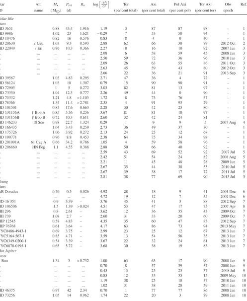
One of the principle ways to split the stellar magnetic energy is into its poloidal and toroidal components which is shown in Fig.2. The top panel shows toroidal magnetic energy density against poloidal magnetic energy density while the bottom panel shows the toroidal energy fraction against stellar mass. Both panels are colour coded by stellar mass aiding comparison between them.
The top panel shows that the toroidal energy is an increasing function of poloidal energy. We can attempt to fit a power law of the formB2
tor ∝ B 2
pola. However, the sample seems to consist of
two sub-samples. The stars with higher magnetic energy densities appear to have a smaller power index,a, than the lower energy stars. A priori, it is not clear which stars should be included in which sub-sample. In the bottom panel, a change of behaviour is evident at approximately 0.5 M. Stars with a larger mass than this can have
at University of St Andrews on November 4, 2015
http://mnras.oxfordjournals.org/
Table 1. Parameters of our sample: star ID, alternative name, stellar mass, rotation period, Rossby number,B2(which is proportional to the magnetic energy density), toroidal magnetic energy (as a percentage of total energy), axisymmetric magnetic energy (as a percentage of total energy), poloidal axisymmetric magnetic energy (as a percentage of poloidal energy), toroidal axisymmetric magnetic energy (as a percentage of toroidal energy) and the observation epoch. Similarly to Vidotto et al. (2014), we have grouped the stars into solar-like stars, young Suns, hot Jupiter hosts and M dwarfs. References indicate the paper where the magnetic map was originally published. For the remaining parameters, references can be found in Vidotto et al. (2014) and references therein.
Star Alt. M Prot Ro log
B2
G2
Tor Axi Pol Axi Tor Axi Obs Ref.
ID name ( M) (d) (per cent total) (per cent total) (per cent pol) (per cent tor) epoch
Solar-like stars
HD 3651 0.88 43.4 1.916 1.19 3 87 87 98 – 1
HD 9986 1.02 23 1.621 −0.29 7 53 50 94 – 1
HD 10476 0.82 16 0.576 0.83 8 4 0 40 – 1
HD 20630 κCeti 1.03 9.3 0.593 2.88 62 66 30 89 2012 Oct 2
HD 22049 Eri 0.86 10.3 0.366 2.27 8 16 10 92 2007 Jan 3
... ... ... ... ... 2.08 6 58 59 45 2008 Jan 3
... ... ... ... ... 2.50 59 72 36 96 2010 Jan 3
... ... ... ... ... 2.09 26 63 55 86 2011 Oct 3
... ... ... ... ... 2.63 45 59 43 80 2012 Oct 3
... ... ... ... ... 2.66 22 36 21 91 2013 Sep 3
HD 39587 1.03 4.83 0.295 2.71 47 36 4 72 – 1
HD 56124 1.03 18 1.307 0.79 15 90 90 91 – 1
HD 72905 1 5 0.272 3.03 82 81 13 97 – 1
HD 73350 1.04 12.3 0.777 2.26 49 44 0 90 – 1
HD 75332 1.21 4.8 >1.105 1.72 8 73 76 37 – 1
HD 78366 1.34 11.4 >2.781 2.35 4 91 93 29 – 1
HD 101501 0.85 17.6 0.663 2.28 30 42 25 80 – 1
HD 131156A ξBoo A 0.85 5.56 0.256 3.67 81 81 10 97 – 1
HD 131156B ξBoo B 0.72 10.3 0.611 2.60 32 42 24 81 – 1
HD 146233 18 Sco 0.98 22.7 1.324 0.29 1 9 9 5 2007 Aug 4
HD 166435 1.04 3.43 0.259 2.73 36 49 37 70 – 1
HD 175726 1.06 3.92 0.272 2.13 24 25 12 68 – 1
HD 190771 0.96 8.8 0.453 2.38 64 75 34 98 – 1
HD 201091A 61 Cyg A 0.66 34.2 0.786 1.05 4 59 58 96 – 1
HD 206860 HN Peg 1.1 4.55 0.388 2.88 50 66 40 92 – 1
... ... ... ... ... 2.59 43 69 52 92 2007 Jul 5
... ... ... ... ... 2.42 51 54 24 82 2008 Aug 5
... ... ... ... ... 2.21 11 45 48 28 2009 Jun 5
... ... ... ... ... 2.67 35 44 38 53 2010 Jul 5
... ... ... ... ... 2.67 39 38 17 72 2011 Jul 5
... ... ... ... ... 2.81 38 77 69 90 2013 Jul 5
Young Suns
AB Doradus 0.76 0.5 0.026 4.92 28 18 9 41 2001 Dec 6
... ... ... ... 4.72 19 12 7 35 2002 Dec 6
BD-16 351 0.9 3.39 – 3.76 45 41 3 88 2012 Sep 7
HD 106506 1.5 1.39 >0.024 4.51 53 47 17 75 2007 Apr 8
HII 296 0.8 2.61 – 3.62 12 36 35 43 2009 Oct 7
HII 739 1.08 2.7 – 2.60 31 33 20 60 2009 Oct 7
HIP 12545 0.58 4.83 – 4.35 35 60 47 83 2012 Sep 7
HIP 76768 0.61 3.64 – 4.17 63 86 73 94 2013 May 7
TYC0486-4943-1 0.69 3.75 – 2.99 23 25 12 67 2013 Jun 7
TYC5164-567-1 0.85 4.71 – 3.59 13 54 56 35 2013 Jun 7
TYC6349-0200-1 0.54 3.39 – 3.67 22 32 24 61 2013 Jun 7
TYC6878-0195-1 0.65 5.72 – 3.68 30 38 19 83 2013 Jun 7
Hot Jupiter hosts
τBoo 1.34 3 >0.732 1.00 63 63 17 90 2008 Jan 9
... ... ... ... 0.70 8 57 59 37 2008 Jun 9
... ... ... ... 0.45 13 25 23 37 2008 Jul 9
... ... ... ... 0.85 12 33 35 15 2009 May 10
... ... ... ... 1.19 38 25 18 37 2010 Jan 10
... ... ... ... 1.02 31 38 28 59 2011 Jan 10
HD 46375 0.97 42 2.34 0.70 1 77 77 86 2008 Jan 10
HD 73256 1.05 14 0.962 1.74 22 20 3 79 2008 Jan 10
at University of St Andrews on November 4, 2015
http://mnras.oxfordjournals.org/
Table 1. –continued
Star Alt. M Prot Ro log
B2
G2
Tor Axi Pol Axi Tor Axi Obs Ref.
ID name ( M) (d) (per cent total) (per cent total) (per cent pol) (per cent tor) epoch
HD 102195 0.87 12.3 0.473 2.22 57 60 23 88 2008 Jan 10
HD 130322 0.79 26.1 0.782 0.81 16 64 58 96 2008 Jan 10
HD 179949 1.21 7.6 >1.726 0.83 18 58 54 78 2007 Jun 11
... ... ... ... 1.13 8 34 34 32 2009 Sep 11
HD 189733 0.82 12.5 0.403 2.69 57 62 26 91 2007 Jun 12
... ... ... ... 3.10 76 77 16 96 2008 Jul 12
M dwarf stars
GJ 569A CE Boo 0.48 14.7 <0.288 4.17 5 96 96 100 2008 Jan 13
GJ 410 DS Leo 0.58 14 <0.267 4.10 82 92 58 99 2007 Jan 13
... ... ... ... ... 4.02 80 78 15 94 2007 Dec 13
GJ 182 0.75 4.35 0.054 4.60 68 66 15 90 2007 Jan 13
GJ 49 0.57 18.6 <0.352 2.94 52 84 67 100 2007 Jul 13
GJ 388 AD Leo 0.42 2.24 0.047 4.77 1 96 97 22 2007 Jan 14
... ... ... ... ... 4.75 3 89 92 8 2008 Jan 14
GJ 494A DT Vir 0.59 2.85 0.092 4.44 62 61 12 91 2007 Jan 13
... ... ... ... ... 4.51 47 49 17 85 2007 Dec 13
GJ 896 A EQ Peg A 0.39 1.06 0.02 5.31 12 66 71 29 2006 Aug 14
GJ 896 B EQ Peg B 0.25 0.4 0.005 5.35 2 92 93 42 2006 Aug 14
GJ 873 EV Lac 0.32 4.37 0.068 5.61 8 31 28 60 2006 Aug 14
... ... ... ... ... 5.48 2 29 29 18 2007 July 14
GJ 1111 DX Cnc 0.1 0.46 0.005 4.14 5 77 77 65 2007 15
... ... ... ... ... 3.85 19 40 30 82 2008 15
... ... ... ... ... 3.83 28 65 61 77 2009 15
GJ 1156 0.14 0.49 0.005 3.71 8 3 2 18 2007 15
... ... ... ... 4.21 11 17 12 57 2008 15
... ... ... ... 4.05 5 1 1 7 2009 15
GJ 1245B 0.12 0.71 0.007 4.59 14 10 6 37 2006 15
... ... ... ... 3.72 9 15 13 30 2008 15
GJ 9520 OT Ser 0.55 3.4 0.097 4.38 33 70 61 90 2008 Feb 13
V374 Peg 0.28 0.45 0.006 5.75 3 79 81 5 2005 Aug 16
... ... ... ... 5.61 3 76 79 2 2006 Aug 16
GJ 412B WX UMa 0.1 0.78 0.008 6.16 2 92 92 89 2006 15
... ... ... ... ... 6.35 2 92 94 38 2007 15
... ... ... ... ... 6.34 2 84 86 3 2008 15
... ... ... ... ... 6.56 3 94 96 20 2009 15
GJ 285 YZ Cmi 0.32 2.77 0.04 5.72 5 57 59 19 2007 Jan 14
... ... ... ... ... 5.66 2 87 88 25 2008 Jan 14
1: Petit (in preparation); 2: do Nascimento et al. (2014); 3: Jeffers et al. (2014); 4: Petit et al. (2008); 5: Boro Saikia et al. (2015); 6: Donati et al. (2003a); 7: Folsom et al. (in preparation); 8: Waite et al. (2011); 9: Fares et al. (2009); 10: Fares et al. (2013); 11: Fares et al. (2012); 12: Fares et al. (2010); 13: Donati et al. (2008b); 14: Morin et al. (2008b); 15: Morin et al. (2010); 16: Morin et al. (2008a).
large toroidal energy fractions but lower mass stars cannot. Though the two panels show essentially the same information, this break in behaviour at 0.5 Mis much clearer in the bottom panel. A num-ber of authors have previously discussed a sudden change in the magnetic properties of M dwarfs at roughly 0.5 M(Donati et al.
2008b; Morin et al.2008b,2010; Gregory et al.2012). They note that this break is roughly coincident with the fully convective limit suggesting a link with the change in internal structure. Dividing our sample on this basis, we find power index values ofa=0.72±0.08 anda=1.25±0.06 for stars less and more massive than 0.5 M, respectively. These power laws are plotted in the top panel with dashed lines. It is worth noting that, among theM<0.5 Mstars, it is the dipole dominate stars that deviate the most from the higher index power law. The non-dipolar stars in the bistable regime, as discussed by Morin et al. (2010), are roughly compatible with the other power law. Additionally, theoretical models predict that these non-dipolar stars can vary cyclically and are able to generate sig-nificant toroidal fields (e.g. Gastine et al.2013).
As a brief aside, we discuss the possibility that the smaller toroidal energy fraction of stars less massive than 0.5 Mis a result of the ZDI technique. ZDI captures the large-scale fields but is insensitive to small-scale fields due to flux cancellation effects. Reiners & Basri (2009) show that the majority of magnetic flux may be missed when the stellar field is reconstructed using only the StokesVsignal when compared to the StokesIsignal. If the lowest mass M dwarfs have a large fraction of their magnetic energy stored in small scale fields, in the form of star-spots for example, these fields may not be reconstructed by the ZDI technique. However, there is no reason to expect ZDI to preferentially miss toroidal field over poloidal field.
It is a well-known observational result that the ratio of X-ray to bolometric luminosity,RX=LX/Lbol, increases with decreasing
Rossby number,Ro, and saturates for stars with Rossby numbers
less than approximately 0.1 (Pizzolato et al.2003; Wright et al.
2011). Here, the Rossby number is defined as the ratio of the stellar rotation period to the convective turnover time. Vidotto et al. (2014) showed that stellar magnetism has the same qualitative dependence
at University of St Andrews on November 4, 2015
http://mnras.oxfordjournals.org/
Figure 1. The rotation periods and masses of each star in our sample. Filled blue points indicate stars observed at one epoch while open red data points indicate stars observed over multiple epochs. Dashed lines are included showing a stellar mass of 0.5 Mand Rossby numbers of 0.01, 0.1 and 1.0.
Figure 2. Top: toroidal magnetic energy against poloidal magnetic energy. Stars with multiple maps are connected by grey lines. The dotted line indi-catesBtor = B2 pol2 . The sample is split into stars less massive (pentagon markers) and more massive than 0.5 M(circle markers). See text for fur-ther discussion of how these sub-samples were chosen. The two dashed lines are best-fitting lines for these sub-samples;B2tor ∝ Bpol2 a with
[image:5.595.49.284.55.238.2]a=0.72±0.08 anda=1.25±0.06 forM<0.5 Mand M>0.5 M, respectively. AB Dor is shown with triangles. Each point is colour coded by stellar mass. Bottom: toroidal energy fraction against stellar mass. Format is the same as the top panel. Data points are also colour coded by stellar mass to aid comparison with the top panel. While the two panels show very similar information, the difference in behaviours of the two mass ranges is much clearer in the bottom panel.
Figure 3. Poloidal (top) and toroidal (bottom) magnetic energy against Rossby number. The formatting is the same as Fig.2. Right/left facing arrows indicate stars that only have lower/upper estimates for their Rossby numbers. The saturated and unsaturated regimes can be clearly seen with the transition occurring at a Rossby number of approximately 0.1. Fits to the stars in the unsaturated regime,Bpol ∝2 R−2.25±0.19
o andBtor ∝2 R−o2.99±0.28, are shown with dashed lines. Note: the magnetic energy axes of the two plots are not the same.
on Rossby number. However, this result was derived using the radial component of the surface fields only, and hence does not consider the toroidal field. In Fig.3, we plot the poloidal (top panel) and toroidal (bottom panel) magnetic energy densities as a function of Rossby number. We use the same Rossby number estimates as Vidotto et al. (2014), where further discussion of the estimates can be found. Left and right facing arrows indicate stars where the Rossby number estimate is only an upper or lower limit, respectively.
It is clear to see that both components qualitatively follow the well-known behaviour with some quantitative differences. In both cases, the cutoff between the saturated and unsaturated regimes oc-curs at Ro∼ 0.1. However, in the saturated regime, the average
magnetic energy of the poloidal fields is higher than that of the toroidal fields by just over an order of magnitude. Additionally, in the unsaturated regime, the slope is steeper for the toroidal com-ponent. The similar behaviour indicates that the same mechanism is responsible for generating both components or that both compo-nents are generated from each other.
Wright et al. (2011) suggested that the difference inRXbehaviour in the saturated and unsaturated regimes can be attributed to different dynamo mechanisms operating in each of the regimes rather than any actual saturation effect. They argued this on the basis that the age at which stars transition from the rotational C sequence to the I sequence (Barnes2003) is coincident with the transition from saturated to unsaturated regimes atRo∼0.1 (see their fig. 4). It
at University of St Andrews on November 4, 2015
http://mnras.oxfordjournals.org/
[image:5.595.56.274.298.593.2]is interesting to note that the majority of the stars in the saturated regime in Fig.3haveM<0.5 M(pentagon symbols). Assuming that the unsaturated stars are those more massive than 0.5 M, we find fits ofB2
pol ∝R−o2.25±0.19andBtor2 ∝Ro−2.99±0.28for the
poloidal and toroidal fields, respectively. These fits are plotted with dashed lines. It is worth noting that these two fits and the fit in Fig.2with the higher power index,a=1.25, are the three possible 2D projections of the same relatively tight sequence of stars in (B2
pol,B 2
tor, Ro) parameter space.
If there is a physical basis for the saturated stars having masses less than 0.5 M, the fact that they appear to have a different power index,a, to the rest of the stars, in Fig.2, is further evidence for the suggestion of Wright et al. (2011). However, care must be taken with this interpretation. Fig.1shows that the majority of stars in our sample that are less than 0.5 Malso have Rossby numbers less than 0.1. Therefore, our interpretation is not that stars in the saturated regime must be less massive than 0.5 M. Rather, it is that stars in the saturated regime are those with Rossby numbers less than∼0.1 which also happen to be stars less massive than 0.5 Min our sample. Noticeably, with the exception of AB Dor (Ro=0.028, M=1.0 M), there is a dearth of stars with Rossby numbers less than ∼0.1 and masses bigger than 0.5 M in our sample. That the lowest mass stars in our sample are also the fastest rotators is not surprising since these stars spin-down less rapidly than higher mass stars (Mohanty & Basri2003). CorrespondinglyRo 0.1, M>0.5 Mstars are harder to find and map. Indeed a number of authors have previously commented on the difficulty in separating stellar mass and Rossby number effects due to this bias (Donati et al.
2008b; Morin et al.2008b,2010; Reiners & Basri2009; Gastine et al.2013). Even when we consider AB Dor (plotted with triangles in Figs2and3), which does fall into theRo0.1,M>0.5 M
region of parameter space, the picture does not become any clearer. In the top panel of Fig.2, AB Dor lies relatively close to both sub-samples such that it is difficult to tell which sub-sample it would be more appropriate for it to be in. Likewise, in Fig. 3, AB Dor falls in an intermediate region. On one hand, one might consider it a saturated star on the basis of its Rossby number which is smaller thanRo∼0.1, the value typically used to delineate the saturated
and unsaturated regimes. However, one might also consider it to be an unsaturated star on the basis that it follows the same trend as the other unsaturated stars, lying at the tail end of that sequence. If the hypothesis of Wright et al. (2011) is correct, one might expect the magnetic fields of the stars in this region of parameter space to obey the power law with the smaller index from Fig.2.
A potential problem with this interpretation is that our two sub-samples were initially chosen on the basis of stellar mass, since this parameter better discriminates between the two power laws in Fig.2, rather than Rossby number. It may be the case that the two power laws in Fig.2do not correspond to the saturated and unsaturated regimes. Indeed, until more stars in theRo<0.1,M> 0.5 M
region of parameter space (corresponding to stars of rotation periods of less than a few days – see Fig.1) have their surface fields mapped, it will be difficult to conclusively confirm or reject this hypothesis. Recently, Reiners, Sch¨ussler & Passegger (2014) reinterpreted the data of Wright et al. (2011). These authors show that, in the unsaturated regime,RX=LX/Lbolshows less scatter when plotted
againstR−4
∗ Prot−2, whereR∗andProtare the stellar radius and rotation
period, respectively, rather than Rossby number, as is traditional in these types of studies. This formulation is approximately equivalent toLX∝P−2
rot, i.e. that X-ray luminosity depends only on the stellar
[image:6.595.311.540.55.239.2]rotation period, in the unsaturated regime. The authors make no claims as to whetherRXas a function ofRoorLXas a function of
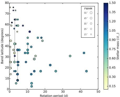
Figure 4. The latitude at which the toroidal azimuthal field peaks for each star as a function of stellar rotation period. Each point is colour coded by stellar mass. The size of the points indicates the full-width half-maximum value for the band (see inset). Stars with multiple maps are connected by grey lines. Numerical values for the data points are included in Table2.
Protis the more physically fundamental relationship. When plotting
B2
polandB 2
toragainstR− 4
∗ Prot−2(not shown), we once again find
that the data separates into saturated and unsaturated regimes. Sim-ilarly to Fig.3, the stars in the saturated regime are those that are less massive than 0.5 M. The suggestion that different dynamo mechanisms are present in the saturated and unsaturated regimes is therefore possible under either interpretation of the rotation-activity relation.
3.2 Band latitudes
In this section, we determine the latitude and extent of azimuthal bands of toroidal field in our sample of stars. First, by examining the magnetic maps, we eliminate those stars that show no evidence of strong bands by determining the fraction of latitudes with only a single polarity in the toroidal component of the azimuthal field. From a visual inspection, stars in which this fraction is less than 0.2 do not have clear bands and we do not attempt to find a band latitude for these stars. For the remaining 67 maps, we average the field strengths over every longitude to obtain an average field strength as a function of latitude and then take the absolute value, i.e.|Btor,φ|(λ), whereλis the latitude. We plot the latitude at which
this function is maximal in Fig.4as a function of rotation period for each star. Stars with maps over multiple epochs are indicated by grey lines. An indication of the band width is given by the full-width half-maximum of the peak in|Btor,φ|(λ). The size of each
data point is scaled by the full width at half-maximum. All points are colour coded by stellar mass. Numerical values for this plot are included in Table2. It is worth highlighting that multiple azimuthal bands of opposing polarity were seen in the rapid rotators HR 1099 and AB Dor (Donati et al.2003b).
Several authors have noted that magnetic flux tends to emerge at higher latitudes on stars with shorter rotation periods as a result of a larger Coriolis force dominating over the magnetic buoyancy of the flux tubes (Schuessler & Solanki1992; Schuessler et al.
1996; Granzer2002). Our results are in qualitative agreement of this statement, with the upper envelope of band latitudes in Fig.4
showing a decreasing trend at longer rotation periods. However, the interplay between Coriolis and buoyancy forces alone cannot
at University of St Andrews on November 4, 2015
http://mnras.oxfordjournals.org/
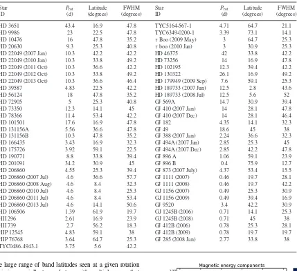
Table 2. Numerical values for Fig.4. For each star the rotation period, latitude of the band and the full-width half-maximum of the band are listed.
Star Prot Latitude FWHM Star Prot Latitude FWHM
ID (d) (degrees) (degrees) ID (d) (degrees) (degrees)
HD 3651 43.4 16.9 47.8 TYC5164-567-1 4.71 64.7 21.1
HD 9986 23 22.5 47.8 TYC6349-0200-1 3.39 73.1 14.1
HD 10476 16 47.8 35.2 τBoo (2009 May) 3 64.7 25.3
HD 20630 9.3 25.3 40.8 τboo (2010 Jan) 3 30.9 25.3
HD 22049 (2007 Jan) 10.3 42.2 42.2 HD 46375 42 33.8 42.2
HD 22049 (2010 Jan) 10.3 33.8 49.2 HD 73256 14 16.9 47.8
HD 22049 (2011 Oct) 10.3 36.6 42.2 HD 102195 12.3 39.4 42.2
HD 22049 (2012 Oct) 10.3 33.8 49.2 HD 130322 26.1 16.9 49.2
HD 22049 (2013 Oct) 10.3 36.6 46.4 HD 179949 (2009 Sep) 7.6 59.1 25.3
HD 39587 4.83 22.5 42.2 HD 189733 (2007 Jun) 12.5 2.8 43.6
HD 56124 18 47.8 35.2 HD 189733 (2008 Jul) 12.5 5.6 52
HD 72905 5 25.3 40.8 GJ 569A 14.7 30.9 39.4
HD 73350 12.3 14.1 45 GJ 410 (2007 Jan) 14 28.1 47.8
HD 78366 11.4 53.4 42.2 GJ 410 (2007 Dec) 14 28.1 46.4
HD 101501 17.6 16.9 47.8 GJ 182 4.35 14.1 32.3
HD 131156A 5.56 36.6 47.8 GJ 49 18.6 45 38
HD 131156B 10.3 47.8 35.2 GJ 388 (2007 Jan) 2.24 36.6 32.3
HD 166435 3.43 16.9 32.3 GJ 494A (2007 Jan) 2.85 25.3 45
HD 175726 3.92 59.1 22.5 GJ 494A (2007 Dec) 2.85 42.2 47.8
HD 190771 8.8 33.8 39.4 GJ 896 A 1.06 59.1 23.9
HD 201091 34.2 30.9 45 GJ 896 B 0.4 75.9 12.7
HD 206860 4.55 25.3 39.4 GJ 873 (2007 July) 4.37 53.4 15.5
HD 206860 (2007 Jul) 4.6 36.6 57.7 GJ 1111 (2007) 0.46 19.7 28.1
HD 206860 (2008 Aug) 4.6 8.4 32.3 GJ 1111 (2008) 0.46 19.7 42.2
HD 206860 (2010 Jul) 4.6 8.4 25.3 GJ 1156 (2007) 0.49 25.3 30.9
HD 206860 (2011 Jul) 4.6 8.4 53.4 GJ 1156 (2009) 0.49 39.4 16.9
HD 206860 (2013 Jul) 4.6 14.1 50.6 GJ 9520 3.4 42.2 30.9
HD 106506 1.39 61.9 19.7 GJ 1245B (2006) 0.71 14.1 25.3
HII 296 2.61 16.9 23.9 GJ 1245B (2008) 0.71 45 38
HII 739 2.7 56.2 18.3 GJ 412B (2006) 0.78 25.3 28.1
HIP 12545 4.83 59.1 38 GJ 412B (2009) 0.78 19.7 19.7
HIP 76768 3.64 64.7 25.3 GJ 285 (2008 Jan) 2.77 33.8 38
TYC0486-4943-1 3.75 5.6 42.2
explain the large range of band latitudes seen at a given rotation period. This is especially true of stars with multiple maps that show the band latitude changing significantly over the course of months/years. In some cases, the azimuthal bands even disappear and reappear between observation epochs.
3.3 Field orientation
From a visual inspection of the magnetic maps, toroidal azimuthal bands appear predominantly axisymmetrically (e.g. Jardine et al.
2013). Fig.5shows the fraction of magnetic energy in axisymmetric modes against the fraction contained in the toroidal component of the field. Mathematically, these correspond to the energy in the m=0 modes1and theγ
, mcoefficients, respectively. Stars with
multiple epochs of observations are connected by grey lines and each point is colour coded by stellar mass. The most striking feature is the dearth of toroidal non-axisymmetric stars, in the lower-right corner of the plot. Additionally, there is no trend evident with stellar mass.
1It is worth noting that an alternative definition of axisymmetric fields,
m< /2, is sometimes used in the literature. This definition encapsulates modes that are nearly aligned with the rotation axis whereas them=0 definition only accounts for modes that are exactly aligned.
Figure 5. Percentage of total magnetic energy contained in the axisym-metric component of the field against percentage of total magnetic energy contained in toroidal field. Stars observed at multiple epochs are connected by grey lines. The data points are colour coded by stellar mass and scale with the total magnetic energy density,B2(see inset). Ros´en, Kochukhov & Wade (2015) reconstructed the surface field of II Peg using StokesIV
(circularly polarized light) and also StokesIQUV(circularly and linearly polarized light). These data points are shown by black diamond and square markers, respectively.
at University of St Andrews on November 4, 2015
http://mnras.oxfordjournals.org/
The striking trend in Fig.5warrants a check for potential biases in the ZDI technique. Cross-talk between the field components, especially the radial and meridional fields is well known and has been characterized (Donati & Brown1997).2In particular, we are
interested in energy from the toroidal field leaking into the poloidal field. To this end, we conducted a systematic series of tests. Specif-ically, we created a grid of synthetic Stokes profiles corresponding to magnetic field geometries where the axisymmetric and toroidal energy fractions ranged from zero to one. Magnetic maps were then reconstructed from these profiles and compared to the original maps that the synthetic profiles were created from. Full details of these tests can be found in Folsom et al. (in preparation). We find that there is some energy leakage from toroidal into poloidal fields (and vice versa). This effect is largest for geometries where the order,, is equal to the degree,mand smallest when there is a large differ-ence betweenandm. However, the effect is not large enough to explain the dearth of points in the lower-right corner of Fig.5.
The magnetic maps used in this study were all reconstructed us-ing the StokesI(unpolarized) and StokesV(circularly polarized) profiles with one exception. Ros´en et al. (2015) observed the star II Peg, during two epochs, in all four Stokes parameters (IQUV; unpolarized, linearly polarized and circularly polarized). They sub-sequently reconstructed magnetic maps using the more commonly used two Stokes profiles (IV) and again using all four. II Peg is plot-ted on Fig.5with black squares and diamonds indicating results obtained using StokesIQUVand StokesIV, respectively. Ros´en et al. (2015) found that the toroidal and axisymmetric energy fractions are similar for both reconstructions though the maps constructed with StokesIQUVcontained significantly more energy than the maps constructed from StokesIV. The latter effect is unsurprising since one should expect more information to be reconstructed, and hence more fields, when using more data. The data points of Ros´en et al. (2015) fall within the trend shown by the rest of the sample. II Peg follows this trend even though it is evolving off the main sequence whereas the rest of the sample are less evolved.
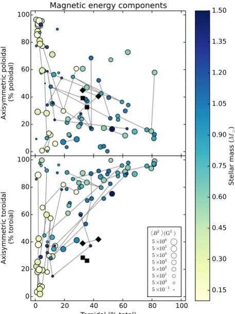
Further insights may be gained by splitting the axisymmetric energy into its poloidal and toroidal components. The top panel of Fig.6shows the fraction of poloidal energy that is axisymmetric, i.e.E(α,m=0,β,m=0)/E(α,m,β,m), against the toroidal energy fraction. The bottom panel of Fig.6is similar but plots the fraction of toroidal energy that is axisymmetric, i.e.E(γ,m=0)/E(γ,m). The formatting is the same as that of Fig.5. As before, the data points of Ros´en et al. (2015) for II Peg are in agreement with the rest of the sample. It is clear that the poloidal and toroidal fields behave differently. While the axisymmetric poloidal energy does not show a clear trend, a clear one is present for the axisymmetric toroidal energy. The data show that toroidal fields are generated in a preferentially axisymmetric manner. This suggests that the toroidal field generation mechanism is sensitive to the rotation axis in a way that the poloidal field is not. Noticeably, there is a cluster of M dwarfs which have dipole dominated fields in the top-left corner of the plot (these are also present in the top left of Fig. 5). Gastine et al. (2013) proposed that the strong dipolar component of these stars inhibits differential rotation and hence the generation of strong toroidal fields through the Omega effect.
[image:8.595.311.540.56.362.2]2In the tests presented by Donati & Brown (1997), the individual field components are considered to be independent parameters. With the new spherical harmonic implementation, as described by Donati et al. (2006), cross-talk is considerably reduced.
Figure 6. Axisymmetric poloidal energy as a percentage of total poloidal energy (top panel) and axisymmetric toroidal energy as a percentage of total toroidal energy (bottom panel) as a function of toroidal energy. Format is the same as Fig.5.
Figure 7. Axisymmetric poloidal energy as a percentage of total poloidal energy against axisymmetric toroidal energy as a percentage of total toroidal energy. Format is the same as Fig.5. Similarly to Fig.5, the inset shows B2values of 5×10⁻¹to 5×10⁶G2in multiples of 10 for the smallest to biggest points. The numerical values are omitted due to lack of space.
We can also consider how the poloidal and toroidal fields are ori-ented with respect to each other. Fig.7plots the fraction of poloidal energy that is axisymmetric against the fraction of toroidal energy that is axisymmetric, i.e. the ordinates of both panels in Fig.6. The data points fill the entire available parameter space for this plot
at University of St Andrews on November 4, 2015
http://mnras.oxfordjournals.org/
[image:8.595.314.533.427.607.2]indicating that the poloidal and toroidal field orientations are not constrained by each other. Alternatively, their orientations may be related to each other but in a complex and non-trivial way. It is particularly interesting that while the orientations of the poloidal and toroidal fields are uncorrelated, there is a relatively tight depen-dence of the toroidal energy density on the poloidal energy density (see Fig.2).
4 C O N C L U S I O N
Over the last decade, large strides have been made in characterizing the strength, geometry and time evolution of cool star magnetic fields. Many stars display strong toroidal azimuthal bands, though currently there is no definitive explanation for their formation. In this paper, we explore the strength and geometry of toroidal magnetic fields by analysing 55 stars that have had their surface magnetic fields mapped with ZDI. This is the first time toroidal fields have been studied in a large sample of stars. The results presented show clear constraints for future dynamo models and can be summarized as follows.
Our sample shows that strong toroidal fields are strongly ax-isymmetric. Conversely, the orientation of poloidal fields are un-constrained with respect to the rotation axis. There is also evidence that the underlying dynamo type affects the relative strength of the poloidal and toroidal fields. We find that stars less massive than 0.5 Mtend to have small toroidal energy fractions while more massive stars can have substantially higher toroidal energy frac-tions. Additionally, the toroidal field energies of the M>0.5 M stars have a steeper power-law dependence on the poloidal field energy than those of the M<0.5 Mstars. These results are in line with the results of Donati et al. (2008b), Morin et al. (2008b,
2010) and Gregory et al. (2012) who noted changes in magnetic properties at 0.5 M, roughly coinciding with the fully convective limit. This suggests some link between the break in magnetic prop-erties with the change in internal structure. These authors also note a strong break in the amount of differential rotation at 0.5 M. It is perhaps telling that the stars with the strongest toroidal fields are those that display differential rotation at their surface. On the other hand, the lowest mass stars, which do not have large toroidal en-ergy fractions (see Fig.2), display little to no differential rotation. This may be a hint that an Omega effect, in the form of differential rotation, is responsible for generating axisymmetric toroidal fields. It would be interesting to compare these observational results to the theoretical dynamo simulations of Brown et al. (2010) and see if their axisymmetry and poloidal/toroidal energy fractions follow the same trends.
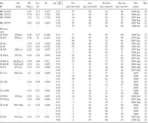
We find that the latitude of the azimuthal bands depends, in part, on the stellar rotation period. On fast rotators, buoyant flux tubes feel a strong Coriolis force and are deflected polewards allowing flux emergence to occur at higher latitudes. Additionally, we find bands at low- to mid-latitudes for all rotation periods. Therefore, rotation period cannot be the only parameter determining the latitude of flux emergence. However, at present, it is unclear what further parameters may be important.
Additionally, we find that the poloidal and toroidal energies both follow the same qualitative behaviour with Rossby number. Both show saturation at low-Rossby number with magnetic energies de-creasing at higher Rossby number. This is also the qualitative be-haviour that X-ray luminosity normalized to bolometric luminosity shows as a function of Rossby number, barring some quantitative differences such as the slope in the unsaturated regime. That the two field components behave similarly indicates that they share a
com-mon generation mechanism or that they are generated from each other. There is evidence that, in our sample, theM<0.5 Mstars correspond to stars in the saturated regime giving credence to the claim of Wright et al. (2011) that stars in the saturated and unsat-urated regimes possess different dynamo mechanisms. However, it remains to be seen whether this is an effect of the bias in our sample. Future spectropolarimetric observations of cool stars withRo0.1, M>0.5 Mwill help confirm or disprove this hypothesis.
AC K N OW L E D G E M E N T S
The authors thank the anonymous referee for their constructive comments. VS acknowledges the support of an Science & Tech-nology Facilities Council (STFC) studentship. AAV acknowledges support from the Swiss National Science Foundation through an Ambizione Fellowship. SBS and SVJ acknowledge research funding by the Deutsche Forchungsgemeinschaft (DFG) under grant SFB, project A16. SGG acknowledges support from the STFC via an Ernest Rutherford Fellowship [ST/J003255/1]. This study was supported by the grant ANR 2011 Blanc SIMI5-6 020 01 ‘Toupies: Towards understanding the spin evolution of stars’ (http://ipag.osug.fr/Anr_Toupies/). This work is based on observa-tions obtained with ESPaDOnS at the CFHT and with NARVAL at the TBL. CFHT/ESPaDOnS are operated by the National Research Council of Canada, the Institut National des Sciences de l’Univers of the Centre National de la Recherche Scientifique (INSU/CNRS) of France and the University of Hawaii, while TBL/NARVAL are operated by INSU/CNRS. We thank the CFHT and TBL staff for their help during the observations.
R E F E R E N C E S
Barnes S. A., 2003, ApJ, 586, 464
Boro Saikia S., Jeffers S. V., Petit P., Marsden S., Morin J., Folsom C. P., 2015, A&A, 573, A17
Brown B. P., Browning M. K., Brun A. S., Miesch M. S., Toomre J., 2010, ApJ, 711, 424
Charbonneau P., 2010, Living Rev. Sol. Phys., 7, 3
Cohen O., Ma Y., Drake J. J., Glocer A., Garraffo C., Bell J. M., Gombosi T. I., 2015, preprint (arXiv:1504.06326)
do Nascimento J. D. et al., 2014, in Petit P., Jardine M., Spruit H. C., eds, Proc. IAU Symp. 302, Magnetic Fields throughout Stellar Evolution. Cambridge Univ. Press, Cambridge, p. 142
Donati J.-F., 1999, MNRAS, 302, 457
Donati J.-F., Brown S. F., 1997, A&A, 326, 1135 Donati J.-F., Collier Cameron A., 1997, MNRAS, 291, 1
Donati J.-F., Collier Cameron A., Hussain G. A. J., Semel M., 1999, MNRAS, 302, 437
Donati J.-F. et al., 2003a, MNRAS, 345, 1145
Donati J.-F., Collier Cameron A., Petit P., 2003b, MNRAS, 345, 1187 Donati J.-F. et al., 2006, MNRAS, 370, 629
Donati J.-F. et al., 2008a, MNRAS, 385, 1179 Donati J.-F. et al., 2008b, MNRAS, 390, 545 Fares R. et al., 2009, MNRAS, 398, 1383 Fares R. et al., 2010, MNRAS, 406, 409 Fares R. et al., 2012, MNRAS, 423, 1006
Fares R., Moutou C., Donati J.-F., Catala C., Shkolnik E. L., Jardine M. M., Cameron A. C., Deleuil M., 2013, MNRAS, 435, 1451
Gastine T., Morin J., Duarte L., Reiners A., Christensen U. R., Wicht J., 2013, A&A, 549, L5
Granzer T., 2002, Astron. Nachr., 323, 395
Gregory S. G., Donati J.-F., Morin J., Hussain G. A. J., Mayne N. J., Hil-lenbrand L. A., Jardine M., 2012, ApJ, 755, 97
Grießmeier J.-M., Zarka P., Spreeuw H., 2007, A&A, 475, 359
at University of St Andrews on November 4, 2015
http://mnras.oxfordjournals.org/
Jardine M., Vidotto A. A., van Ballegooijen A., Donati J.-F., Morin J., Fares R., Gombosi T. I., 2013, MNRAS, 431, 528
Jeffers S. V., Petit P., Marsden S. C., Morin J., Donati J.-F., Folsom C. P., 2014, A&A, 569, A79
Llama J., Wood K., Jardine M., Vidotto A. A., Helling C., Fossati L., Haswell C. A., 2011, MNRAS, 416, L41
Marsden S. C. et al., 2011, MNRAS, 413, 1922 Mohanty S., Basri G., 2003, ApJ, 583, 451
Morgenthaler A., Petit P., Morin J., Auri`ere M., Dintrans B., Konstantinova-Antova R., Marsden S., 2011, Astron. Nachr., 332, 866
Morgenthaler A. et al., 2012, A&A, 540, A138 Morin J. et al., 2008a, MNRAS, 384, 77 Morin J. et al., 2008b, MNRAS, 390, 567
Morin J., Donati J.-F., Petit P., Delfosse X., Forveille T., Jardine M. M., 2010, MNRAS, 407, 2269
Petit P. et al., 2008, MNRAS, 388, 80
Petit P., Dintrans B., Morgenthaler A., Van Grootel V., Morin J., Lanoux J., Auri`ere M., Konstantinova-Antova R., 2009, A&A, 508, L9
Pizzolato N., Maggio A., Micela G., Sciortino S., Ventura P., 2003, A&A, 397, 147
Reiners A., Basri G., 2009, A&A, 496, 787
Reiners A., Sch¨ussler M., Passegger V. M., 2014, ApJ, 794, 144 Ros´en L., Kochukhov O., Wade G. A., 2015, ApJ, 805, 169
Schuessler M., Solanki S. K., 1992, A&A, 264, L13
Schuessler M., Caligari P., Ferriz-Mas A., Solanki S. K., Stix M., 1996, A&A, 314, 503
See V., Jardine M., Vidotto A. A., Petit P., Marsden S. C., Jeffers S. V., do Nascimento J. D., 2014, A&A, 570, A99
See V., Jardine M., Fares R., Donati J.-F., Moutou C., 2015, MNRAS, 450, 4323
Vidotto A. A., Fares R., Jardine M., Donati J.-F., Opher M., Moutou C., Catala C., Gombosi T. I., 2012, MNRAS, 423, 3285
Vidotto A. A., Jardine M., Morin J., Donati J.-F., Lang P., Russell A. J. B., 2013, A&A, 557, A67
Vidotto A. A. et al., 2014, MNRAS, 441, 2361
Vidotto A. A., Fares R., Jardine M., Moutou C., Donati J.-F., 2015, MNRAS, 449, 4117
Waite I. A., Marsden S. C., Carter B. D., Hart R., Donati J.-F., Ram´ırez V´elez J. C., Semel M., Dunstone N., 2011, MNRAS, 413, 1949 Wright N. J., Drake J. J., Mamajek E. E., Henry G. W., 2011, ApJ, 743, 48 Zarka P., 2007, Planet. Space Sci., 55, 598
This paper has been typeset from a TEX/LATEX file prepared by the author.
at University of St Andrews on November 4, 2015
http://mnras.oxfordjournals.org/