Modelling the hidden magnetic field of low mass stars

Modelling the hidden magnetic field of low-mass stars

P. Lang,

M. Jardine,

J. Morin,

J.-F. Donati,

S. Jeffers,

A. A. Vidotto

and R. Fares

1_{SUPA, School of Physics and Astronomy, University of St Andrews, North Haugh, St Andrews KY16 9SS, UK} 2_{Institut f¨ur Astrophysik, Friedrich-Hund-platz 1, D-370777 G¨ottingen, Germany}

3_{Dublin Institute for Advanced Studies, School of Cosmic Physics, 31 Fitzwilliam Place, Dublin 2, Ireland} 4_{IRAP-UMR 5277, CNR and Univ. de Toulouse, 14 Av. E. Belin, F-31400 Toulouse, France}

5_{University of Utrecht, PO Box 80000, NL-3508 TA Utrecht, the Netherlands}

Accepted 2014 January 14. Received 2014 January 9; in original form 2013 August 26

A B S T R A C T

Zeeman–Doppler imaging is a spectropolarimetric technique that is used to map the large-scale surface magnetic fields of stars. These maps in turn are used to study the structure of the stars’ coronae and winds. This method, however, misses any small-scale magnetic flux whose polarization signatures cancel out. Measurements of Zeeman broadening show that a large percentage of the surface magnetic flux may be neglected in this way. In this paper we assess the impact of this ‘missing flux’ on the predicted coronal structure and the possible rates of spin-down due to the stellar wind. To do this we create a model for the small-scale field and add this to the Zeeman–Doppler maps of the magnetic fields of a sample of 12 M dwarfs. We extrapolate this combined field and determine the structure of a hydrostatic, isothermal corona. The addition of small-scale surface field produces a carpet of low-lying magnetic loops that covers most of the surface, including the stellar equivalent of solar ‘coronal holes’ where the large-scale field is opened up by the stellar wind and hence would be X-ray dark. We show that the trend of the X-ray emission measure with rotation rate (the so-called ‘activity–rotation relation’) is unaffected by the addition of small-scale field, when scaled with respect to the large-scale field of each star. The addition of small-scale field increases the surface flux; however, the large-scale open flux that governs the loss of mass and angular momentum in the wind remains unaffected. We conclude that spin-down times and mass-loss rates calculated from surface magnetograms are unlikely to be significantly influenced by the neglect of small-scale field.

Key words: stars: activity – stars: coronae – stars: low-mass – stars: magnetic field – X-rays: stars.

1 I N T R O D U C T I O N

M dwarfs, much smaller, dimmer and cooler than stars like our Sun, are by far the most common type of star in our Galaxy. The study of these stars has remained limited due to their faintness and in the past it was presumed that M dwarfs were unlikely to host detectable habitable planets. More recently however, the advantages of search-ing for habitable planets around M dwarfs have been recognized. For example, the habitable zone is closer and so it is easier to find planets by radial velocity searches. Despite the advantages of de-tecting planets around these stars, M dwarfs have been shown to be extremely magnetically active which may have significant effects on any planetary system. For example, intense magnetic fields, stellar flares, ultraviolet (UV) and X-ray emission and the powerful stellar

E-mail:pl42@st-andrews.ac.uk

winds (Vidotto et al.2013) may affect planetary atmospheres as well as any potential organisms on these planets. This makes it vital to investigate how the structure and evolution of the magnetic field, both large-scale and small-scale, can affect coronal properties.

Time-resolved spectropolarimetric observations of a star can be analysed by means of Zeeman–Doppler imaging (ZDI; Semel1989; Donati et al.2006b) in order to reconstruct a map of the vector magnetic field on the stellar surface. ZDI relies on the fact that due to the combination of the properties of the Zeeman effect, e.g. rotation-induced Doppler and rotational modulation, a strong relation exists between the distribution of the magnetic field at the surface of a star and the rotational evolution of polarization in spectral lines during a stellar rotation. However, several limitations exist: in particular, with the solution being non-unique, a maximum entropy criterion has to be used, and due to the mutual cancellation of polarized signals originating from neighbouring regions of opposite polarities, the maps have a limited spatial resolution and, therefore, systematically

2014 The Authors

at University of St Andrews on September 9, 2014

http://mnras.oxfordjournals.org/

miss magnetic flux corresponding to magnetic fields organized on small spatial scales. The actual resolution is mostly driven by the rotational velocity of the star projected on the observer’s line-of-sight (vsini): the higher thevsini, the higher the resolution. In addition, for the inclination of the stellar rotation axis with respect to the line-of-sight differing from 90◦, a part of the star is never visible. Therefore, in that region there is no constraint on the magnetic field, except that globally it has to satisfy the null-divergence constraint. Studies based on spectropolarimetric observations and ZDI have provided the first information on the structure of the surface mag-netic fields of M dwarfs. In particular, partly convective M dwarfs have been shown to host large-scale magnetic fields which are non-axisymmetric and feature a strong toroidal component (Donati et al.

2008), whereas those close to the limit of full convection have been shown to host much stronger large-scale field dominated by a mainly axisymmetric poloidal component (e.g. Donati et al.2006a; Morin et al.2008a,b). However, these studies do not constrain the small-scale field component of the magnetic fields of low-mass stars. In parallel, studies based on the analysis of the Zeeman broadening in unpolarized spectroscopy provide complementary information: the measure of the disc-averaged magnetic field including the contribu-tions of both the large-scale and small-scale components. Reiners & Basri (2009) compiled measurements of mean magnetic flux from StokesI (total intensity) and Stokes V (the fractional degree of circular polarization) parameters for a selection of partially con-vective and fully concon-vective M dwarfs. They find that the fraction of magnetic flux visible in StokesVis a small percentage of the total flux measured in StokesI. This means that a large portion of the magnetic flux stored in magnetic fields is invisible to StokesV. One possible explanation is that the majority of magnetic flux on M dwarfs is grouped into small structures distributed over the stellar surface, where different polarities cancel each other out in StokesV. More specifically, Reiners & Basri (2009) find that although for the lower mass fully convective stars, the mean magnetic flux does not significantly differ from partially convective stars (Reiners & Basri

2007), the fraction of the total magnetic flux detected in StokesV

is different for partially convective and fully convective stars: 6 and 14 per cent, respectively.

The aim of this paper is to determine the influence that this small-scale field might have on the stellar coronae. We create a model for small-scale field and add it to the reconstructed surface radial maps for a stellar sample of 12 M Dwarfs (Donati et al.2008; Morin et al.

2008b) that span the fully convective boundary. By comparison with the observed large-scale magnetic field structure, we investigate the effect this small-scale field has on the geometry of the extrapolated 3D magnetic field and subsequent coronal properties, such as open flux, coronal extent, X-ray emission measure and coronal density. We approach this in two ways: (1) by incorporating small-scale field that has the same surface distribution and magnitude on to each star in the sample; and (2) using the results of Reiners & Basri (2009), we add in a percentage amount of small-scale field such that the large-scale field contributes only 6 and 14 per cent of the total magnetic field, for the partially convective and fully convective stars within the sample, respectively.

2 M O D E L L I N G A N D I N C O R P O R AT I N G T H E S M A L L - S C A L E F I E L D

2.1 The surface field

To create small-scale field on the stellar surface we use the syn-thesized spot brightness maps of Barnes, Jeffers & Jones (2011).

The spots were created using the Doppler imaging code ‘Doppler Tomography of Stars’ (DoTS) and all spots were modelled, following

Solanki (1999), with circular umbral areas and a ratio of umbral to penumbral area of 1:3.

We use the spot brightness to allocate field strengths to the centre of the active regions and allow the field strength to fall-off in a Gaussian-like distribution, to the edge of each spot, i.e.

Bss r =

Bmax

brightness

e−x

2

2, ₍₁₎

where Bss

r represents the field strength in the small-scale field,

brightnessis the spot brightness,Bmaxis the arbitrarily chosen

maxi-mum field strength andxis the distance from the centre of the spot. We note here that a higher spot brightness indicates a lower field strength value.

We impose a condition that the small-scale field must be small enough not to be detected in ZDI, i.e. invisible in StokesV. The typical area over which the circular polarization cancels out e.g. the area over which the signed magnetic flux cancels or the typical distance between two spots of opposite polarities, corresponds to about 12◦, for a rapidly rotating star withvsini≈40 km s−1_e.g.

V374 Peg. This condition means that any active region must have a diameter less than the typical ZDI resolution, i.e.<5◦. Our synthetic maps assume spots with radii≤1◦.

To ensure the small-scale field is evenly distributed over the entire surface of the star, we keep the spot coverage constant. We, therefore, find that an appropriate parameter to vary in the model isBmax. Taking into account the magnitude of the field detected

in ZDI for our sample of partly convective and fully convective M Dwarfs, we (1) fix the value of Bmax to be either ±500 G or ±1000 G; and (2) set the value ofBmax such that the large-scale

field contributes between approximately 6 and 14 per cent of the total field, respectively, as indicated in Reiners & Basri (2009). The values for the average radial flux in each case can be found in Table1.

The surface magnetic radial map for the small-scale field is shown in Fig.1where the spot distribution covers approximately 62 per cent of a model star. Fig.1represents the case whereBmax=500 G.

The simulated magnetic radial maps for the small-scale field are added to the reconstructed radial maps obtained through ZDI and new surface maps with both large-scale and small-scale field are created for each M dwarf, i.e.BTotal=Brss+B

ls r.

2.2 The coronal field

The magnetic field is extrapolated above the stellar surface using the potential field source surface (PFSS) method (Altschuler & Newkirk

1969), where the magnetic field is assumed to be current free (∇ ×

B=0) and divergence free (∇ ·B=0). In a format similar to Jardine et al. (1999) the components for the coronal magnetic field are determined from the solution to Laplace’s equation∇2_{ψ =0,}

whereψis the scalar potential:

Br= − N

l=1 l

m=1

lalmrl−1−(l+1)blmr−(l+2)Plm(cosθ)eimφ, (2)

Bθ = − N

l=1 l

m=1

almrl−1+blmr−(l+2) d

dθPlm(cosθ)e

imφ_{, (3)}

Bφ = − N

l=1 l

m=1

almrl−1+blmr−(l+2)Plm(cosθ)_sinim_θeimφ, (4)

at University of St Andrews on September 9, 2014

http://mnras.oxfordjournals.org/

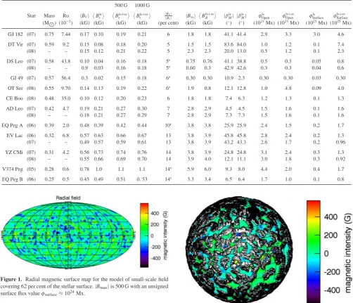
Table 1. Values for mass, radius, Rossby number andBV(the average large-scale magnetic flux derived from spectropolarimetric measurements) are from Donati et al. (2008) and Morin et al. (2008b). Values ofBV

BI for GJ 182, DT Vir, Ce Boo, AD Leo, EV Lac and YZ CMi are from Reiners & Basri (2009), while values for DS Leo, GJ 49, OT Ser EQ Peg A, V374 Peg and EQ Peg B are estimates (depicted bye_{) based on Reiners & Basri (2009). Values for}

Bls

r(the average large-scale [ls] radial flux),Bss(the average small-scale [ss] flux, scaled with respect to the large-scale field) andBls+ss(the average

large-scale+small-scale flux) as well asφOpen(the open flux) andφSurface(the surface flux) values are from this work.

500 G 1000 G Star Mass Ro BV

Bls r

Bls+ss r Blsr+ss

BV

BI Bss

Bls+ss

R |βMls| |βlsM| φOpenls φ ls+ss

Open φSurfacels φ

ls+ss Surface

(M ) (10−2_{) (kG) (kG) (kG) (kG) (per cent) (kG) (kG) (}◦_{) (}◦_{) (10}23_{Mx) (10}23_{Mx) (10}25_{Mx) (10}25_Mx)

GJ 182 (07) 0.75 7.44 0.17 0.10 0.19 0.21 6 1.8 1.8 41.1 41.4 2.9 3.3 3.0 4.6

DT Vir (07) 0.59 9.2 0.15 0.08 0.18 0.20 5 1.5 1.5 83.6 84.0 1.0 1.2 0.1 7.4

(08) – – 0.15 0.12 0.21 0.22 5 2.3 2.3 20.0 13.0 0.5 1.2 0.1 2.3

DS Leo (07) 0.58 43.8 0.10 0.04 0.16 0.18 5e _{0.75 0.76 41.1 38.8 0.5 0.3 0.05 0.8}

(08) – – 0.9 0.03 0.16 0.18 5e _{0.60 0.3 42.9 42.6 0.3 0.3 0.04 0.6}

GJ 49 (07) 0.57 56.4 0.3 0.02 0.15 0.18 6e _{0.30 0.30 10.9 2.3 0.30 0.30 0.03 0.30}

OT Ser (08) 0.55 9.70 0.14 0.13 0.19 0.22 6e _{1.9 0.8 12.1 12.8 1.0 4.8 0.09 4.0}

CE Boo (08) 0.48 35.0 0.10 0.12 0.20 0.23 6 1.8 1.8 7.4 6.3 1.2 1.3 0.1 1.3

AD Leo (07) 0.42 4.7 0.19 0.21 0.27 0.30 7 2.8 2.9 4.5 4.5 1.5 1.6 0.1 1.6

(08) – – 0.18 0.21 0.27 0.29 7 2.8 2.9 7.3 7.3 1.5 1.6 0.1 1.6

EQ Peg A (06) 0.39 2.0 0.48 0.39 0.42 0.44 10e _{3.8 3.8 25.9 25.9 2.4 1.5 0.2 1.7}

EV Lac (06) 0.32 6.8 0.57 0.63 0.66 0.67 13 3.8 3.9 45.8 45.8 2.8 2.4 0.2 1.3

(07) – – 0.49 0.57 0.59 0.61 13 3.8 3.9 43.2 43.3 2.6 1.7 0.2 0.96

YZ CMi (07) 0.31 4.2 0.56 0.73 0.74 0.76 14 3.8 3.9 24.8 24.8 3.1 2.4 0.3 1.3

(08) – – 0.55 0.66 0.69 0.70 14 3.9 4.0 12.1 11.1 3.0 1.8 0.3 0.92

V374 Peg (05) 0.28 0.6 0.78 1.0 1.1 1.1 14e _{5.9 6.0 9.3 8.0 4.4 2.0 0.4 1.7}

EQ Peg B (06) 0.25 0.5 0.45 0.49 0.51 0. 53 14e _{3.3 3.4 6.5 6.4 1.7 1.0 0.1 0.8}

Figure 1. Radial magnetic surface map for the model of small-scale field covering 62 per cent of the stellar surface.|Bmax|is 500 G with an unsigned

surface flux valueφsurface≈1024Mx.

withBr,B_θandB_φrepresenting the radial, meridional and azimuthal components of the magnetic field, respectively,Plmrepresents the associated Legendre polynomials,almandblmare the amplitudes of the spherical harmonics,lis the spherical harmonic degree,mis the order or azimuthal number andr=R/R.

To extrapolate the 3D coronal field and determine the amplitude of the spherical harmonics,alm andblm, we apply two boundary conditions. The upper condition is that at the source surface,Rss

(Schatten, Wilcox & Ness1969), the field opens and is purely radial (B_θ=B_φ=0), while the lower boundary condition imposes the ob-served radial field. We choose the solar value for the source surface at 2.5R_∗. The code used to extrapolate the field is a modified ver-sion of the global diffuver-sion model developed by van Ballegooijen, Cartledge & Priest (1998). The extrapolated 3D small-scale field is shown in Fig.2, where the field lines remain closed and close to the stellar surface. This extrapolation demonstrates that the small-scale field produces a ‘carpet’ of low-lying loops across the surface.

Figure 2. 3D coronal extrapolation of the small-scale field shown in Fig.1. Colours are scaled to the maximum and minimum values of the surface radial magnetic field component.

2.3 X-ray emission model

The structure of the magnetic field is influenced by the strength of the surface field and the distribution of plasma. Following the model in Lang et al. (2012), the density structure can be estimated for the extrapolated corona by assuming the plasma is hydrostatic and isothermal and that the gas pressure at the stellar surface is proportional to the magnetic pressure (po=κBo2).κis a constant

of proportionality relating the base gas pressurepo to magnetic

pressureBothrough the magnetic constant 2μ. The value ofκ is

chosen such that the coronal densities lie within the observed range for M dwarfs, 109_–1012_cm−3 _{(Ness et al. 2002, 2004). Typical}

values for logκ=[−5:−7].

at University of St Andrews on September 9, 2014

http://mnras.oxfordjournals.org/

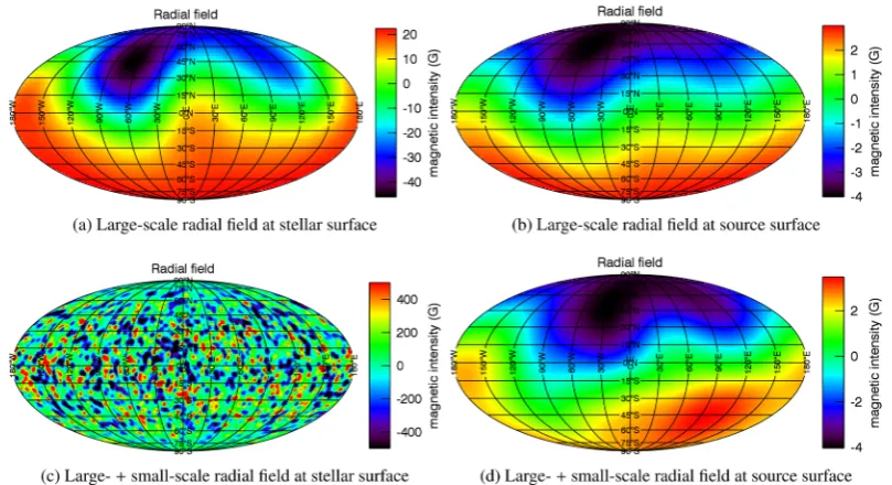
Figure 3. Upper: large-scale (ZDI) reconstructed radial field maps for GJ 49 at (a) the stellar surface, and (b) the source surface. Lower: ZDI+small-scale radial field map for GJ 49 at (c) the stellar surface, and (d) the source surface. Small-scale field is scaled according to the results of Reiners & Basri (2009) such thatBls=6 per centBTotal, for partly convective M dwarfs.

We assume that the pressure varies along each field line according to

p=poe

g·Bds

|B| , ₍₅₎

as described by Jardine et al. (2002) and Gregory et al. (2006). Expanding the (dimensionless) component of gravity along the field line (g·B), we have

p=κB2 oexp

⎡ ⎣

−φg

r2 +φcrsin2θ

Br+(φcrsinθcosθ)Bθ

B2

r+Bθ2+Bφ2

ds ⎤ ⎦_,

(6)

wherer=R/Rand the ratios of centrifugal (φc) and gravitational

(φg) to thermal energy are given by

φc=me

(ωR)2

kBT

, (7)

φg=me

GM

RkBT

, (8)

whereRis the stellar radius,Mis the stellar mass,ωis the stellar rotation rate,kB is the Boltzmann constant,Gis the gravitational

constant andmeis the electron mass.

To ensure that only regions of the closed stellar corona con-tribute towards the emission measure, the gas pressure along open field lines is taken to be zero. In addition to this, if there is any overpressure along the designated closed loops, i.e. gas pressure (p=2nekT)≥magnetic pressure (pB=B2/2μ), then the pressure

at that grid point is also set to zero.

Assuming the gas is optically thin, the X-ray emission measure varies with density, i.e.

EM(r)=

n2

edV . (9)

The temperature (T=2×106_{K), source surface (R}

ss=2.5R∗)

and constant of proportionalityκ(10−6_{) are kept constant in this}

paper (for more details see Lang et al.2012).

3 R E S U LT S

3.1 Field structure

With the addition of small-scale field B drops more rapidly with height, close to the stellar surface. As such, we do not find any great change in the large-scale field structure. This is evident from Fig.3which shows the radial field at both the stellar surface and the source surface. Figs3(a) and (c) which represent the large-scale and large-scale+small-scale field at the stellar surface, respectively, show very different topologies; however, when this is extrapolated out to the source surface (Figs3b and d) the topologies are similar. We conclude from this that the magnetic pressure falls off with radius more quickly with the addition of small-scale field leaving only the large-scale components near the source surface.

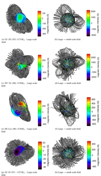
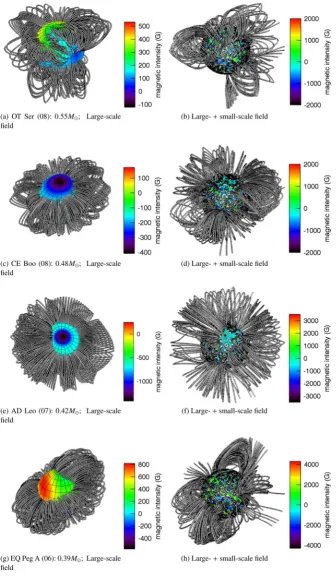
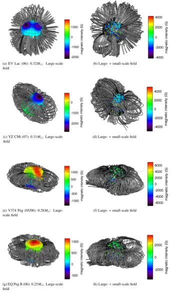
Fig.4shows the coronal magnetic field of (1) the large-scale field extrapolated from the reconstructed radial maps (left-hand column); and (2) the large-scale+scale field, where the small-scale field is small-scaled according to Reiners & Basri (2009), such that

Bls = 6 per centBTotal, for partly convective M dwarfs andBls =

14 per centBTotal, for fully convective M dwarfs (right-hand

col-umn). A comparison of the extrapolations in both the left- and right-hand columns from Fig.4shows the location of coronal holes where the stellar wind is emitted and the angle of the magnetic dipole axis from the rotation pole remain largely unchanged on the majority of the stars in the sample. However, the extrapolations of DT Vir, OT Ser and EQ Peg A show small changes in the structure of the closed large-scale field.

3.2 Activity–rotation relation

The X-ray luminosity has been shown to correlate well with either rotational velocity or Rossby number Ro (the ratio of the stellar

at University of St Andrews on September 9, 2014

http://mnras.oxfordjournals.org/

Figure 4. Column (1) shows the 3D coronal extrapolation for the reconstructed surface radial maps for our sample of M dwarfs. Column (2) is the extrapolation for case (2) with the combination of the small-scale field scaled with respect to the large-scale field e.g.Bls=6 per centBTotal, for the partly convective M

dwarfs andBls=14 per centBTotal, for the fully convective M dwarfs.

at University of St Andrews on September 9, 2014

http://mnras.oxfordjournals.org/

Figure 4 – continued

rotation period,P, to the convective turnover time,τc; e.g. Pizzolato

et al.2003a,b; Jeffries et al.2011); in general,LX/Lbolincreases and

then saturates (LX/Lbol≈10−3; Delfosse et al.1998) with

increas-ing rotation rate. This behaviour is attributed to coronal saturation (Vilhu & Walter1987; Stauffer et al.1994) and occurs at Ro ≈ 0.1. For a sample of M dwarfs, Lang et al. (2012) reproduce the

saturation of the X-ray emission measure for the large-scale field detected through ZDI. These results are shown in Figs5and6as black symbols.

With the addition of small-scale field, the correlation between the X-ray emission measure and Rossby number changes depend-ing on the amount of small-scale flux added. For case (1), shown

at University of St Andrews on September 9, 2014

http://mnras.oxfordjournals.org/

Figure 4 – continued in Fig.5, the rise and saturation of the X-ray emission measure is

not as prominent with the addition of 500 G of small-scale flux (red symbols) and is no longer evident for 1000 G of small-scale flux (blue symbols). This means that adding the same surface distribution of small-scale field to each star destroys the relationship between magnetic flux and Rossby number. If we now consider case (2)

whereBls =6 per centBTotal, for the partly convective M dwarfs,

and Bls = 14 per centBTotal, for the fully convective M dwarfs

shown in Fig.6, the rise and saturation of the X-ray emission with Rossby number is once again apparent. The magnitude of the X-ray emission has increased by approximately five orders of magnitude due to the increase in flux (Table2).

at University of St Andrews on September 9, 2014

http://mnras.oxfordjournals.org/

Figure 5. X-ray emission measure as a function of Rossby number for both the large-scale field (black symbols) and the simulated small-scale+ large-scale field (Bmax =500 G, red symbols;Bmax =1000 G, blue symbols).

Symbols: asterisks represent partly convective dwarfs,M>0.4 M , and diamond represents fully convective dwarfs,M≤0.4 M .

Figure 6. X-ray emission measure as a function of Rossby number for both the large-scale field (black symbols) and the simulated small-scale+ large-scale field (purple symbols). Symbols: asterisks represent partly convective dwarfs,M> 0.4 M , and diamond represents fully convective dwarfs, M≤0.4 M .

For comparison with our previous work (Lang et al.2012) con-ducted on the field visible only to ZDI, we keep the model pa-rameters e.g. the temperature (T = 2 ×106_{K), source surface}

(Rss=2.5R∗) andκ=10−6, constant. Keepingκconstant results

in an increase in pressure and coronal density due to the increase in the surface flux. The coronal densities (shown in Table2) now lie at the higher end of the accepted range: 109_–1012_cm−3_{(Ness et al.}

2002,2004), as opposed to their previous values which were at the lower end. The value ofκcould be altered in such a way to reduce the coronal densities back to the values calculated for the ZDI maps and in turn reduce the magnitude of the X-ray emission measure.

Comparison of the results of Figs 5 and 6 indicates that the addition of the same small-scale field to each star removes the activity–rotation relation; however, scaling the small-scale field to the large-scale, e.g.Bls=6 per centBTotal, for the partly convective

M dwarfs andBls= 14 per centBTotal, for the fully convective M

dwarfs, recovers the relation. This would suggest that the small-scale field has the same dependence on rotation period as the large-scale field. Our results are in agreement with that of Garraffo et al. (2013) who find that the small-scale field structure (of similar spatial resolution) plays a crucial role when modeling the closed loop structure.

In our previous work (Lang et al.2012), the rotational modula-tion of the X-ray emission measure for the stellar sample did not demonstrate any trend with Rossby number and could not be used as an indicator of field topology due to too many contributing factors e.g. the angle of stellar inclination and the angle of the magnetic dipole axis from the rotation pole. We find that with the addition of small-scale field, both with the same surface distribution and magnitude, and scaled with respect to the large-scale field, this is still the case.

With the addition of small-scale field, the magnitude of the ro-tation modulation of the X-ray emission measure changes for each star as a result of changes in surface field strength (see Table2). For OT Ser, an early M dwarf, the change in the rotational modulation between the large-scale field and the addition of small-scale flux is nearly 30 per cent, whereas for GJ 49, also an early M dwarf, the change in the modulation is 1 per cent. Since we do not find any great change in the large-scale field structure with the addition of

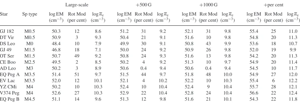
Table 2. Results for the coronal properties for the sample of M dwarfs. The predicted values for the logarithmic emission measure (both magnitude, log EM, and rotational modulation, Rot Mod) and logarithmic coronal density, logne, for the observed large-scale field, are from Lang et al. (2012). The

logarithmic emission measure (both magnitude, log EM, and rotational modulation, Rot Mod) and logarithmic coronal density, lognefor the simulated

large-scale+small scale field atBmax=500 and 1000 G as well as forBls=6 per centBTotalfor partly convective stars andBls=14 per centBTotalfor

fully convective stars, are from this work.

Large-scale +500 G +1000 G +per cent

Star Sp type log EM Rot Mod logne log EM Rot Mod logne log EM Rot Mod logne log EM Rot Mod logne

(cm−3) (per cent) (cm−3) (cm−3) (per cent) (cm−3) (cm−3) (per cent) (cm−3) (cm−3) (per cent) (cm−3)

GJ 182 M0.5 50.3 12 8.6 51.2 31 9.2 52.1 31 9.8 55.4 25 11.0

DT Vir M0.5 50.9 3 9.3 50.4 21 9.1 51.6 10 9.8 54.8 20 11.3

DS Leo M0 48.4 10 7.9 49.9 30 9.1 50.8 43 9.9 53.6 18 10.7

GJ 49 M1.5 46.8 18 7.1 50.0 24 9.2 50.9 26 9.8 52.0 19 9.9

OT Ser M1.5 50.7 49 9.2 50.8 24 9.3 51.6 13 9.8 54.2 20 11.3

CE Boo M2.5 49.5 2 8.5 50.2 4 9.2 51.3 10 9.7 54.9 20 11.4

AD Leo M3 50.2 3 8.9 50.6 0.4 9.4 50.6 0.4 9.4 54.5 10 11.7

EQ Peg A M3.5 51.4 51 9.7 51.5 44 9.7 51.8 48 10.0 54.9 27 12.0

EV Lac M3.5 52.0 12 10.1 52.1 4 10.2 52.2 10 10.3 55.4 6 12.2

YZ CMi M4 50.2 10 10.3 52.4 10 10.4 52.4 9 10.4 55.7 28 12.1

V374 Peg M4 52.6 27 10.3 52.9 22 10.4 52.8 24 10.4 56.6 22 12.4

EQ Peg B M4.5 51.1 14 9.6 51.3 12 9.8 51.6 21 10.1 54.3 22 11.8

at University of St Andrews on September 9, 2014

http://mnras.oxfordjournals.org/

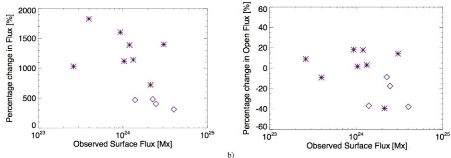
Figure 7. The percentage change in (a) the surface flux and (b) the open flux as a function of the observed surface flux due to the addition of small-scale field. Symbols are as of Fig.5.

small-scale field, the change in the magnitude of the rotational mod-ulation could be a result of the small-scale field producing low-lying small closed field regions which carpet the stellar surface including the areas where the large-scale field is open.

3.3 Open flux and spin-down

Coronal structure is important as it determines the X-ray emission from regions of closed magnetic field but also areas where the mag-netic field is open and the stellar wind forms. For stars with weaker large-scale magnetic fields, the range of field strengths presents on the star has been altered by the addition of small-scale field. This has little effect on the geometry of the large-scale field (Fig.4). The dipole axis and the location and extent of the open field regions are largely unchanged. This is to be expected as the small-scale field is distributed axisymmetrically over the surface so it has no preferred direction. This suggests that the latitudes from which a stellar wind could be launched would not be affected by the presence of small-scale field. Within regions where the large-small-scale field is open there may still be a carpet of small-scale field, which could contribute to powering the stellar wind (e.g. Nishizuka et al.2011).

The stellar wind is responsible for angular momentum loss and influences the stellar spin-down time. To investigate the effect the small-scale field has on the overall coronal structure, we examine both its influence on the total magnetic flux at the surface of the star and also the total open flux. We analyse the geometry of the field by predicting and comparing the open flux to observed surface flux values obtained from the overall combination oflandmmodes:

Open

Surface = R2ss

|Br(Rss, θ, φ)|d

R2

∗

|Br(R∗, θ, φ)|d,

(10)

whereis the solid angle. We note this gives a lower limit to the true open flux as on some field lines the gas pressure may exceed the magnetic pressure.

Adding in small-scale field increases the surface flux. Fig.7(a) shows this increase expressed as

φSurface=

(φSurface)large+small

(φSurface)large

−1. (11)

The fractional increase in surface flux is clearly greatest for those stars whose large-scale surface flux is lowest.

The addition of the small-scale field also results in a slight change (10–40 per cent) in the open flux (Fig.7b) but shows no preference

between partly convective and fully convective stars. The fraction for the open flux is given by

φOpen=

(φOpen)large+small

(φOpen)large

−1. (12)

This result is in keeping with the increase in surface flux, which would increase the magnetic pressure (equation 5). We note that the magnitude of the open flux is dependent on the chosen value for the source surface (asRss=→ ∞,Open→0) but the effect of

adding in small-scale field is the same for all values of the source surface. As there is little change in the open flux with the addition of small-scale field, we would not expect the angular momentum or mass loss to be significantly affected. These results agree with the MHD-model used by Garraffo et al. (2013).

For many stars a full surface magnetic map is not available and only a single flux estimate is possible. Assuming that all of the surface flux is contained in one single mode, for example a dipole, can however lead to an overestimate of the amount of open flux. As discussed in Lang et al. (2012), the open flux for any single mode is simply related to the surface flux as

Open

Surface =

(2l+1)

Rss R∗

l+1

l+(l+1)

Rss R∗

2l+1. (13)

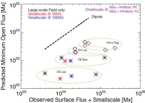
Fig.8shows that when small-scale field is added there is an increase in surface flux but the predicted open flux is still at least an order of magnitude smaller than it would be had we only considered the dipole modes. Therefore, the angular momentum loss, ˙J, due to the stellar wind, which is determined by the amount of open flux, i.e. a Weber–Davis model (Weber & Davis1967), given by

˙

J∝2

Open (14)

is influenced by the topology of the field and would be overestimated by at least two orders of magnitude. This is also true for the mass-loss rate,

˙

M∝Open, (15)

which could be overestimated by an order of magnitude if the topol-ogy is oversimplified. We conclude from this result that when pro-ducing a model for the stellar corona, or the stellar wind, a range of

landmmodes must be considered to reproduce the correct, more complex, coronal structure.

at University of St Andrews on September 9, 2014

http://mnras.oxfordjournals.org/

Figure 8. Comparison of the magnitude of the minimum predicted open flux as a function of the observed surface flux with and without small-scale field. The dashed line shows the predicted open flux of a pure dipole. Four stars which span the spectral range of our sample have been chosen to show that when producing a model for the stellar corona a range oflandmmodes must be considered to reproduce the correct coronal structure. Symbols are as of Fig.5.

4 S U M M A RY

We have created a model for small-scale field using synthesized spot distribution maps. We allocate field strengths in a Gaussian distribution from the centre of the spot by either (1) fixing the value ofBmaxto be either±500 G or±1000 G; or (2) setting the value

ofBmaxsuch that the large-scale field contributes only 6 per cent of

the total field for partly convective M dwarfs and 14 per cent of the total field for fully convective M dwarfs, as indicated in Reiners & Basri (2009). We have incorporated the radial surface map produced by this model into the reconstructed maps of the observed radial magnetic field at the stellar surface for a sample of early-to-mid M dwarfs and extrapolated their 3D coronal magnetic field using the PFSS method.

We have investigated the effect the addition of small-scale field has on the topology of the large-scale magnetic field at the stellar surface and the structure of the extrapolated 3D corona. By assuming a hydrostatic, isothermal corona, we have determined the following.

(1) The geometry of the magnetic field e.g. the angle of the dipole axis, overall large-scale structure of the 3D extrapolated corona and location of coronal holes where the stellar wind is emitted all remain largely unchanged.

(2) Addition of the same small-scale field to each star removes theLX−Ro relation; however, scaling the small-scale field to the

large-scale (ZDI) field recovers the relation. We conclude from this that the small-scale field has the same dependence on rotation period as the large-scale field.

(3) The magnitude of the rotational modulation of the X-ray emission measure changes with the addition of more surface flux; however, no trend with Rossby number Ro is found. This change could be due to the carpet of low-lying field.

(4) The addition of small-scale field increases the surface flux. (5) And finally, we find that the large-scale open flux does not vary greatly with the addition of small-scale field. This suggests that

the mass-loss rate, the angular momentum loss and the spin-down time for a star are not significantly affected by small-scale flux.

AC K N OW L E D G E M E N T S

PL acknowledges support from a Science and Technology Facili-ties Council studentship. JM, AAV and RF acknowledge support from fellowships of the Alexander von Humboldt foundation, the Royal Astronomical Society and Science and Technology Facilities Council, respectively. The authors would like to thank the referee for a particularly thorough and detailed report.

R E F E R E N C E S

Altschuler M. D., Newkirk G., 1969, Sol. Phys., 9, 131

Barnes J. R., Jeffers S. V., Jones H. R. A., 2011, MNRAS, 412, 1599 Delfosse X., Forveille T., Perrier C., Mayor M., 1998, A&A, 331, 581 Donati J.-F., Forveille T., Collier Cameron A., Barnes J. R., Delfosse X.,

Jardine M. M., Valenti J. A., 2006a, Science, 311, 633 Donati J.-F. et al., 2006b, MNRAS, 370, 629

Donati J.-F. et al., 2008, MNRAS, 390, 545

Garraffo C., Cohen O., Drake J. J., Downs C., 2013, ApJ, 764, 32 Gregory S. G., Jardine M., Collier Cameron A., Donati J.-F., 2006, MNRAS,

373, 827

Jardine M., Barnes J. R., Donati J.-F., Collier Cameron A., 1999, MNRAS, 305, L35

Jardine M., Wood K., Collier Cameron A., Donati J.-F., Mackay D. H., 2002, MNRAS, 336, 1364

Jeffries R. D., Jackson R. J., Briggs K. R., Evans P. A., Pye J. P., 2011, MNRAS, 411, 2099

Lang P., Jardine M., Donati J.-F., Morin J., Vidotto A., 2012, MNRAS, 424, 1077

Morin J. et al., 2008a, MNRAS, 384, 77 Morin J. et al., 2008b, MNRAS, 390, 567

Ness J.-U., Schmitt J. H. M. M., Burwitz V., Mewe R., Raassen A. J. J., van der Meer R. L. J., Predehl P., Brinkman A. C., 2002, A&A, 394, 911 Ness J.-U., G¨udel M., Schmitt J. H. M. M., Audard M., Telleschi A., 2004,

A&A, 427, 667

Nishizuka N., Nakamura T., Kawate T., Singh K. A. P., Shibata K., 2011, ApJ, 731, 43

Pizzolato N., Maggio A., Micela G., Sciortino S., Ventura P., 2003a, in Brown A., Harper G. M., Ayres T. R., eds, The Future of Cool-Star Astrophysics: 12th Cambridge Workshop on Cool Stars, Stellar Systems, and the Sun. University of Colorado, Boulder, p. 887

Pizzolato N., Maggio A., Micela G., Sciortino S., Ventura P., 2003b, A&A, 397, 147

Reiners A., Basri G., 2007, ApJ, 656, 1121 Reiners A., Basri G., 2009, A&A, 496, 787

Schatten K. H., Wilcox J. M., Ness N. F., 1969, Sol. Phys., 6, 442 Semel M., 1989, A&A, 225, 456

Solanki S. K., 1999, in Butler C. J., Doyle J. G., eds, ASP Conf. Ser. Vol. 158, Solar and Stellar Activity: Similarities and Differences. Astron. Soc. Pac., San Francisco, p. 109

Stauffer J. R., Liebert J., Giampapa M., Macintosh B., Reid N., Hamilton D., 1994, AJ, 108, 160

van Ballegooijen A. A., Cartledge N. P., Priest E. R., 1998, ApJ, 501, 866 Vidotto A. A., Jardine M., Morin J., Donati J.-F., Lang P., Russell A. J. B.,

2013, A&A, 557, A67

Vilhu O., Walter F. M., 1987, ApJ, 321, 958 Weber E. J., Davis L., Jr, 1967, ApJ, 148, 217

This paper has been typeset from a TEX/LA_{TEX file prepared by the author.}

at University of St Andrews on September 9, 2014

http://mnras.oxfordjournals.org/