ISSN Online: 2160-0503 ISSN Print: 2160-049X
DOI: 10.4236/wjm.2019.912018 Dec. 19, 2019 267 World Journal of Mechanics
Elastic Collisions in Minkowski Momentum
Space with Lorentz Transformations
Akihiro Ogura
Laboratory of Physics, Nihon University, Matsudo, Japan
Abstract
We reexamined the elastic collision problems in the special relativity for both one and two dimensions from a different point of view. In order to obtain the final states in the laboratory system of the collision problems, almost all text-books in the special relativity calculated the simultaneous equations. In con-trast to this, we make a detour through the center-of-mass system. The two frames of references are connected by the Lorentz transformation with the velocity of the center-of-mass. This route for obtaining the final states is easy for students to understand the collision problems. For one dimensional case, we also give an example for illustrating the states of the particles in the Min-kowski momentum space, which shows the whole story of the collision.
Keywords
Relativistic Elastic Collision, Minkowski Momentum Space, Lorentz Transformation
1. Introduction
Collisions of the interacting particles have fundamental importance in both clas-sical mechanics and special relativity. Illustrating the collision problems is re-warding to understand them clearly and quickly.
For one dimensional collision in classical mechanics, mass-momentum dia-gram plays a key role [1] [2]. We can see the whole story of the collision in the single diagram for both the center-of-mass and the laboratory systems. For two dimensional collision in classical mechanics, two-dimensional momentum space describes the collision clearly in the textbook [3]. We also see the slightly differ-ent illustration which lays emphasis on the transformation of the two systems [4]. For one dimensional collision in the special relativity, Saletan [5] proposed to understand the collision problems in the Minkowski momentum space, with How to cite this paper: Ogura, A. (2019)
Elastic Collisions in Minkowski Momen-tum Space with Lorentz Transformations. World Journal of Mechanics, 9, 267-284.
https://doi.org/10.4236/wjm.2019.912018
Received: November 15, 2019 Accepted: December 16, 2019 Published: December 19, 2019
Copyright © 2019 by author(s) and Scientific Research Publishing Inc. This work is licensed under the Creative Commons Attribution International License (CC BY 4.0).
DOI: 10.4236/wjm.2019.912018 268 World Journal of Mechanics energy E/c represented along the vertical axis and momentum p represented along the horizontal axis. The states of the particles are expressed by the arrow in the space. The quantitative application of it is stated by [6]. We do not need any calculation for obtaining the whole story of the collision. For two dimen-sional collision in the special relativity, illustration is clearly stated in the litera-ture [6] [7]. We also see the slightly different illustration which lays emphasis on the transformation of the two systems [8].
In this article, we propose a different point of view for the elastic collision problems in the special relativity. We make a detour through the center-of-mass system for obtaining the final states in the laboratory system. It is applicable to both one and two dimensional collisions. This method shows the unified way to think about collision problems.
Now, consider two reference frames K and K'. We assume that the frame K'
moves in the x-direction at speed V with respect to the frame K. And let us as-sume the origins O and O' of the two reference frames coincide at time t=0. An event that occurs at some point is observed from both frames and is charac-terized by a set of coordinates
(
ct x y z, , ,)
and(
ct x y z′ ′ ′ ′, , ,)
where c is the speed of light. The Lorentz transformation gives the relation between two coor-dinates and it is described by0 0 0 0
,
0 0 1 0
0 0 0 1
γ
βγ
βγ
γ
′ −
′ −
=
′
′
ct ct
x x
y y
z z
(1)
where β =V c and
γ
=1 1−β
2 . In the following paper, we designate the frame K as the laboratory system, while K' as the center-of-mass system. Accor-dingly, the velocity V describes the velocity of the center-of-mass. The inverse transformation is given by just putting −β to β in Equation (1).Our strategy is pictorially stated in Figure 1. In the textbooks of physics, we have to calculate the simultaneous equations of momentum- and ener-gy-conservation in order to obtain the final states in the laboratory system. See the dashed arrow in Figure 1. Our strategy is as follows.
1) By the Lorentz inverse transformation, we obtain the velocity V of the cen-ter-of-mass in terms of energies (EA, EB) and momenta (pA, pB) in the
la-boratory system before the collision. The velocity V does not change throughout the collision.
2) By the Lorentz transformation, we obtain the momenta ( ∗ A
p , ∗ B
p ) in the center-of-mass system before the collision. See the strategy 2 in Figure 1. In this frame, two particles make a head on collision with the same magnitude of the momentum p∗.
3) We determine the momenta ( ′∗ A
p , ′∗ B
p ) in the center-of-mass system after
DOI: 10.4236/wjm.2019.912018 269 World Journal of Mechanics
Figure 1. The usual approach to the collision problems is along the dashed arrow. The strategy in this article is on the detour of the solid arrows.
4) By the Lorentz inverse transformation, we obtain the momenta (p′A, p′B)
in the laboratory system after the collision. See the strategy 4 in Figure 1. Finally, we reach the final states. We never solve the simultaneous equations in contrast with the usual treatment of the collision problems.
5) Let us consider the two special cases. One is that the target particle is at rest (pB =0) in the laboratory system before the collision. The other is that, in ad-dition to the conad-dition above, two particles have equal masses.
6) We check the limit c→ ∞ and see whether these strategies recover the Newtonian mechanics.
This paper is organized in the following way. In Section 2, we discuss one di-mensional collisions, according to the strategy stated above. We also show the illustration of these collisions in Minkowski momentum space. This diagram shows the whole story of the one dimensional collision in the special relativity. In Section 3, we turn to the two dimensional collision case. We introduce the collision angle θ∗ of the incident particle in the center-of-mass system. We show the theoretical background for the diagrammatic approach [6][7] [8]. Sec-tion 4 is devoted to a summary.
2. Elastic Collisions in One Dimension
Let us discuss the one dimensional elastic collisions. The motions of the particles are restricted in the x-direction. Therefore, the y- and z-components of the mo-mentum are zero. Although the illustrations of the contents of this section are already done by [5] [6], we reexamined how we draw the collision problems in the Minkowski momentum space.
2.1. Velocity of Center-of-Mass System
DOI: 10.4236/wjm.2019.912018 270 World Journal of Mechanics transformation with the whole two body system,
0 0 0 0
.
0 0 1 0
0 0
0 0 0 1
0 0
γ βγ βγ γ
∗ ∗
∗ ∗
+
+
+ = +
A B A B
A B A B
E E E E
c c c c
p p p p (2)
Here, ∗+ ∗ =0
A B
p p is the definition of the center-of-mass system. From the matrix, we obtain the following relations:
,
βγ ∗ ∗
+ = +
A B
A B E E
p p
c c (3)
.
γ ∗ ∗
+ = +
A B A B
E E E E
c c c c (4)
Dividing these equations, we obtain the velocity of the center-of-mass
,
β = = + + A B A B
p p
V
E E
c
c c
(5)
which is conserved throughout the collision because of the conservation law of energy and momentum. Moreover, we define the following conserved quantity:
(
)
2 2
2, ∗ ∗
≡ + = + − +
A B A B
A B
E E E E
s p p
c c c c (6)
2 2 2 2 2 ,
= + + −
A B
A B E E A B
m c m c p p
c c (7)
where mA and mB are the masses of the colliding particles. We used the
rela-tion
(
E c)
2−p2=( )
mc 2, which is satisfied by the relativistic particle. When we define W as the total energy in the center-of-mass system, then W is written in terms of s as follows:. ∗ ∗ ≡ A+ B =
W E E c s (8) We also calculate the following quantities from Equation (5),
2
1 , ,
1
γ βγ
β
+ +
= = =
−
A B
A B
E E
p p
c c
s s (9)
[image:4.595.268.449.93.162.2]which are frequently used in the following sections.
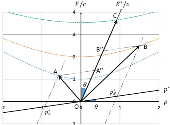
Figure 2 depicts the states of two particles before the collision in the labora-tory system:
, ,0,0 , , ,0,0 .
= =
OA A OB B
A B
E p E p
c c (10)
DOI: 10.4236/wjm.2019.912018 271 World Journal of Mechanics
Figure 2. Figure shows the case in [6]: mA=1, vA= −0.5c, mB=2,
0.6 = B
v c. The tips A and B show the states of the particles before the col-lision in the laboratory system. The tip C is determined from A and B by the parallelogram law.
of the perfect inelastic collision in the special relativity, i.e., the two particles are combined and move with the velocity β after the collision. Contrary to this, this diagram is also interpreted as the decay process. The parent particle OC decays into two daughter particles OA and OB.
2.2. Momenta and Energies in the Center-of-Mass System before
the Collision
We discuss the strategy 2 in the Introduction. Concerning the Lorentz transfor-mation for each particle,
0 0 0 0
0 0 0 0
, ,
0 0 1 0 0 0 0 1 0 0
0 0
0 0 0 1 0 0 0 0 1 0
0 0
γ βγ γ βγ
βγ γ βγ γ
∗ ∗
∗ ∗
− −
− −
= =
A B
A B
A B
A B
E E
E E
c c
c c
p p
p p (11)
we obtain the momenta in the center-of-mass system before the collision;
,
βγ γ
∗ = − + = + −
B A
A B
A
A A
E E
p p
E c c
p p
c s (12)
,
βγ γ
∗ = − + = − −
B A
A B
B
B B
E E
p p
E c c
p p
c s (13)
where we used Equations (9). It is natural that ∗+ ∗ =0
A B
DOI: 10.4236/wjm.2019.912018 272 World Journal of Mechanics ,
∗≡ − = ∗ = − ∗
B A
A B
A B
E E
p p
c c
p p p
s (14)
for later use. The energies of the particles in the system are also given by Equa-tions (11),
2 2
2 2 2 2 , 2
γ βγ
∗ − + + −
= − = =
A B
A B A
A A A B
A
E E p p m c
E E p c c s m c m c
c c s s (15)
2 2
2 2 2 2 , 2
γ βγ
∗ − + − +
= − = =
A B
A B B
B B A B
B
E E p p m c
E E p c c s m c m c
c c s s (16)
where we used Equations (7) and (9). These energies are also derived by
( )
2 2 2∗ = ∗ +
A A
E c p m c and ∗ =
( )
∗ 2+ 2 2B B
E c p m c with Equations (12) and (13). Summing up these energies, we can easily see Equation (8).
We obtain these results from Figure 3. We draw a new p∗-axis which has the slope tanθ with respect to the horizontal p-axis. Drawing the dotted line from the tips A and B to the p∗-axis in parallel to the line OC, the crossing points indicate the momenta ∗
A
p and ∗ B
p whose distances from the origin O are equal. This means ∗+ ∗ =0
A B
p p . Moreover, we draw the dotted line from the tips
A and B to the line OC in parallel to the p∗-axis. The crossing points A'' and B'' describe the energies ∗
A
E c and ∗ B
E c in the center-of-mass system before the collision.
2.3. Momenta and Energies in the Center-of-Mass System after the
Collision
[image:6.595.234.511.472.675.2]We discuss the strategy 3 in the Introduction. We determine the momenta in the
DOI: 10.4236/wjm.2019.912018 273 World Journal of Mechanics center-of-mass system after the collision. In this frame, the particles move in the opposite direction after the collision with the same magnitude of p∗ in Equa-tion (14). We write down the momenta in the center-of-mass system after the collision
, .
∗ ∗ ∗ ∗ ∗ ∗
′ ≡ − = − ′ ≡ − = +
A A B B
p p p p p p (17)
Since the magnitudes of the momenta do not change, the energies of the par-ticles
,
∗ ∗ ∗ ∗
′ = ′ =
A A B B
E E E E (18)
do not change either in this frame, where ∗ A
E and ∗ B
E are given by equations (15) and (16).
2.4. Momenta and Energies in the Laboratory System after the
Collision
We discuss the strategy 4 in the Introduction. Consider the Lorentz inverse transformation for each particle,
0 0 0 0
0 0 0 0
, ,
0 0 1 0 0 0 1 0
0 0 0 0
0 0 0 1 0 0 0 1
0 0 0 0
γ βγ γ βγ
βγ γ βγ γ
∗ ∗
∗ ∗
′ ′ ′ ′
′ = ′ ′ = ′
A A B B
A A B B
E E E E
c c c c
p p p p (19)
we obtain the momenta in the laboratory system after the collision. From the second row of these matrices, we obtain
2 2
,
βγ ′∗ γ ∗
′ = + ′
− + + −
+
= × − ×
A
A A
A B A B B A
A B A A B
A B
E
p p
c
E E p p m c E E p E p E
p p c c c c c c
s s s s
(20)
2 2
,
βγ ′∗ γ ∗
′ = + ′
− + + −
+
= × + ×
B
B B
A B A B B A
A B B A B
A B
E
p p
c
E E p p m c E E p E p E
p p c c c c c c
s s s s
(21)
where we used Equations (9), (17) and (18). Adding the two equations, we easily see the conservation of momentum: p′A+p′B = pA+pB. Moreover, we also ob-tain the energies from Equations (19),
2 2
,
γ ∗ βγ ∗
′ ′ ′
= +
+ − + + −
= × − ×
A A
A
A B A B B A
A B A A B
A B
E E p
c c
E E E E p p m c p E p E
p p
c c c c c c
s s s s
DOI: 10.4236/wjm.2019.912018 274 World Journal of Mechanics 2 2
,
γ ∗ βγ ∗
′ = ′ + ′
+ − + + −
= × + ×
B B
B
A B A B B A
A B B A B
A B
E E p
c c
E E E E p p m c p E p E
p p
c c c c c c
s s s s
(23)
where we used Equations (9), (17) and (18). We easily check the conservation of energy: E′A +E′B = EA+EB
c c c c .
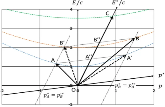
Figure 4 shows the whole story of the one dimensional collision. Since the momenta of the particles exchange in the center-of-mass system after the colli-sion, the tips A and B', B and A' are on the same dotted line. Thus, the dashed vectors
, ,0,0 , , ,0,0
′ ′
′= ′ ′= ′
OA A OB B
A B
E p E p
c c (24)
show the states after the collision. Namely, the tip A(B) can slide on the
hyper-bola
(
( ))
( ) ( )2 2 2 2
− =
A B A B A B
E c p m c until the tip A'(B'). Furthermore, the sum of these vectors OA OB′+ ′ equals OC, which means that OC is not altered throughout the collision.
The point A''(B'') is the midpoint of the line AA'(BB') which means that the energies in the center-of-mass system do not change before and after the colli-sion, i.e., Equation (18).
Once the momenta and energies of the particles before the collision are given, we obtain the final states as shown in Figure 4 without any calculations.
2.5. In Case of
p
B=
0
We discuss the strategy 5 in the Introduction. In this case, we substitute 2
= B B
[image:8.595.233.515.512.695.2]E m c into the equations of this section. Equation (7) becomes simple form
DOI: 10.4236/wjm.2019.912018 275 World Journal of Mechanics
2 2 2 2 2 ,
= + + A
A B B E
s m c m c m c
c (25) and we obtain the relation
.
βγ ∗ γ ∗
+
= =
A
B A B
B
E m c p m c
E p c
c s (26)
From Equations (20) and (21), we obtain the momenta in the laboratory system after the collision
2 2 2 2 2
,
+
−
′ = × = − ×
A
B B
A B
A A A A
E
m c m c
m c m c c
p p p p
s s (27)
2
.
+
′ = ×
A
B B
B A
E
m c m c
c
p p
s (28)
The second term of the right hand side of Equation (27) is a momentum lost by the particle A, and this transfers to the momentum gained by the particle B in Equation (28). This is the impulse in the special relativity. We obviously under-stand the conservation of the momentum: p′A+p′B = pA. In addition, we obtain the energies from Equations (22) and (23)
2
2 ,
′
= − ×
A A B
A
E E m c p
c c s (29)
2
2 .
′
= + ×
B B
B A
E m c m c p
c s (30)
The second terms of the right hand side of both equations are the same and it transfers from the particle A to B. This is the work in the special relativity. The sum of these energies ′A+ B′ = A+
B
E E E m c
c c c shows the conservation law of
[image:9.595.253.499.207.288.2]energy.
Figure 5 shows the Minkowski momentum diagram in this case. The vector OB is along the vertical axis, which means pB =0 before the collision.
2.6. In Case of
p
B=
0
and
m
A=
m
B=
m
The quantity s becomes more simple form
2 ,
= +
A
E
s mc mc
c (31) and we obtain the following relations
. 2
βγ EA∗ =βγ E∗B =γp∗ = pA
c c (32)
We obtain the momenta
0, ,
′ = ′ =
A B A
p p p (33)
DOI: 10.4236/wjm.2019.912018 276 World Journal of Mechanics
Figure 5. The solid and dashed arrows show the states of the particles be-fore and after the collision in case of pB=0.
, ,
′ ′
= =
A B A
E mc E E
c c c (34)
in the laboratory system. After the collision, the incident particle A stops and the initially rest particle B moves with the momentum of which the particle A had before the collision.
2.7. In the Limit
c→ ∞In the limit c→ ∞, the relativistic energy E is replaced by mc2. Equation (5) becomes
.
+ + +
= → =
+ +
+
A B A B A B
A B A B A B
p c p c p c p c p p
V E E
m c m c m m
c c
(35)
This is the velocity of the center-of-mass in Newtonian mechanics. Equation (7) shows
(
)
22 2 2 2 2 2 2 2 ,
→ A + B + A B − A B= A+ B − A B
s m c m c m cm c p p m m c p p (36)
then, the Lorentz factors Equations (9) become
(
)
2 2 2(
)
2 2 2 1,γ → + = + →
+ − + −
A B A B
A B A B A B A B
m c m c m m
m m c p p m m p p c
(
)
2 2 2 0.βγ→ + →
+ −
A B
A B A B
p p
m m c p p
Equation (14) becomes
(
)
2 2 2(
)
2 2 2,
∗→ − = −
+ − + −
− →
+
A B B A A B B A
A B A B A B A B
B A A B
A B
p m c p m c p m p m
p
m m c p p m m p p c
m p m p
m m
DOI: 10.4236/wjm.2019.912018 277 World Journal of Mechanics which is the momentum in the center-of-mass system in Newtonian mechanics. Using these equations, we obtain the momenta Equations (20) and (21),
,
∗
+ −
′ → − = −
+ +
A B B A A B
A A A
A B A B
p p m p m p
p m m V p
m m m m (38)
,
∗
+ −
′ → + = +
+ +
A B B A A B
B B B
A B A B
p p m p m p
p m m V p
m m m m (39)
after the collision in the laboratory system, which are recovered the case in Newtonian mechanics.
3. Elastic Collisions in Two Dimensions
Let us turn our discussion to the case of the two dimensional elastic collisions. We suppose that the motions of the particles are restricted in the x-y plain, so that the z-component of the momentum is zero. Since the motions of the par-ticles are supposed along the x-direction before the collision, we repeat the same discussion of Subsections 2.1 and 2.2. The illustration of this section is already done by [7] [8].
3.1. Momenta and Energies in the Center-of-Mass System after
the Collision
Let us start our discussion from the strategy 3 in the Introduction. In the cen-ter-of-mass system, the magnitudes of the momenta do not change before and after the collision. Thus, we write down the momenta in the same way with Equ-ation (14),
, ∗≡ − = ∗ = ∗ = ′∗ = ′∗
B A
A B
A B A B
E E
p p
c c
p p p p p
s (40)
where s is defined by Equation (7).
However, the direction of the momenta changes after the collision in two di-mensions. As shown in Figure 6, we define the sense of the momentum p′∗
A as
(
cos ,sin ,0θ
θ
)
∗= ∗ ∗
n , where θ∗ is the scattering angle of the particle A in the center-of-mass system. In other words, the momenta after the collisions are de-noted by the vector-form:
. ∗ ∗ ∗ ∗
′ = = − ′
pA p n pB (41) Since the magnitudes of the momenta do not change in this frame throughout the collision, the energies of each particle do not change either:
, ,
∗ ∗ ∗ ∗
′ = ′ =
A A B B
E E E E (42)
where ∗ A
E and ∗ B
E are given by Equations (15) and (16).
3.2. Momenta and Energies in the Laboratory System after the
Collision
DOI: 10.4236/wjm.2019.912018 278 World Journal of Mechanics
Figure 6. Left: The collision in the center-of-mass system. The scattering angles θ∗ and
φ∗ have the relation θ∗+φ∗= π. Right: The collision in the laboratory system.
written by p′A =
(
p p′Ax, ′Ay,0)
=(
pA′cos ,θ
p′Asin ,0θ
)
and(
, ,0)
(
cos ,φ
sin ,0φ
)
′ = ′ ′ = ′ − ′
pB p pBx By pB pB , where θ and φ are the scattering
angle of the particles A and B in the laboratory system as shown in Figure 6. From the Lorentz inverse transformation, we obtain the momenta in the la-boratory system after the collision by using Equation (41)
0 0 0 0
cos cos ,
0 0 1 0
sin sin
0 0 0 1
0 0 0
γ βγ βγ γ
θ θ
θ θ
∗
∗ ∗
∗ ∗
′ ′
′ = ′ =
′ ′
A A A
Ax A
Ay A
E E E
c c c
p p p
p p p
(43)
0 0 0 0
cos cos .
0 0 1 0
sin sin
0 0 0 1
0 0 0
γ βγ βγ γ
φ θ
φ θ
∗
∗ ∗
∗ ∗
′ ′
′ = ′ = −
′ − ′ −
B B B
Bx B
By B
E E E
c c c
p p p
p p p
(44)
From the second and third row of these matrices, we obtain x- and
y-components of the momentum for the particle A,
cosθ βγ ∗ γ ∗cos ,θ∗
′ = ′ = A+
Ax A E
p p p
c (45)
sinθ ∗sin ,θ∗
′ = ′ =
Ay A
p p p (46)
and for the particle B,
cosφ βγ ∗ γ ∗cos ,θ∗
′ = ′ = B−
Bx B E
p p p
c (47)
sinφ ∗sin .θ∗
′ = − ′ = −
By B
p p p (48)
Combining with the relation cos2θ∗+sin2θ∗ =1, we obtain 2
2 1,
βγ γ
∗
∗ ∗
′ −
′
+ =
A
Ax E Ay
p p
c
DOI: 10.4236/wjm.2019.912018 279 World Journal of Mechanics 2 2 1. βγ γ ∗ ∗ ∗ ′ − ′ + = B
Bx E By
p p
c
p p (50)
These equations show the ellipse with the following parameters:
minor semiaxis ∗= − ,
B A
A E B E
p p
c c
p
s (51)
major semiaxis γ ∗ ,
+ −
=
A B B A
A B
E E p E p E
c c c c
p
s (52)
(
)
eccentricity βγ ∗ ,
+ −
=
B A
A B A E B E
p p p p
c c
p
s (53)
(
)
2 2midpoint of foci βγ ∗ ,
+ − +
=
A B
A B A B A
A
E E
p p p p m c
E c c
c s (54)
(
)
2 2midpoint of foci βγ ∗ ,
+ − +
=
A B
A B A B B
B
E E
p p p p m c
E c c
c s (55)
where Equations (7), (9), (14), (15) and (16) are used.
From the Lorentz transformation Equation (43) with Equation (15), we obtain the energy in the laboratory system after the collision
(
)
cos
cos
1 cos ,
γ βγ θ
γ γ βγ βγ θ
βγ θ ∗ ∗ ∗ ∗ ∗ ∗ ∗ ′ = + = − + = − − A A A A A
E E p
c c
E p p
c
E p
c
(56)
where we used Equations (9). In the same manner, from Equations (44) and (16), we obtain
(
)
cos
cos
1 cos .
γ βγ θ
γ γ βγ βγ θ
βγ θ ∗ ∗ ∗ ∗ ∗ ∗ ∗ ′ = − = − − = + − B B B B B
E E p
c c
E p p
c
E p
c
(57)
The second terms of the right hand side in Equations (56) and (57) show the energy lost by the particle A and the energy gained by the particle B. This is the work in the special relativity. From these energies, we clearly see the conserva-tion law of the energy: E′A +EB′ = EA +EB
DOI: 10.4236/wjm.2019.912018 280 World Journal of Mechanics
3.3. In Case of
p
B=
0
We discuss the strategy 5 in the Introduction. The parameters of the ellipse be-come simple form:
minor semiaxis p∗ = p m cA B ,
s (58)
major semiaxis γ ∗ βγ ∗,
+
= =
A
B A B
B
E m c p m c
E c
p
s c (59)
2 eccentricity βγp∗= p m cA B ,
s (60)
2 2
midpoint of foci βγ ∗ ,
+
=
A
A B A
A
E
p m c m c
E c
c s (61)
where s is given by Equation (25). Equation (59) is as the same relation with Eq-uation (26). The ellipse EqEq-uation (49) with these parameters is depicted in Fig-ure 7. This is already done by [8].
3.4. In Case of
p
B=
0
and
m
A=
m
B=
m
The parameters of the ellipse are the followings:
minor semiaxis p∗= p mcA ,
s (62)
major semiaxis ,
2
γp∗ = pA =βγ E∗B
c (63)
eccentricity ,
2
βγ ∗= − A
E mc
c
p (64)
midpoint of foci ,
2
βγ E∗A = pA
c (65)
where s is given by Equation (31). Equations (63) and (65) are as same as Equa-tion (32).
Dividing Equations (45), (46) and Equations (47), (48), we obtain the relations of the scattering angles
sin sin
tan ,
1 cos cos
θ
θ γ
θ
θ
βγ
γ
θ
∗ ∗ ∗
∗ ∗
∗ ∗
= =
+ +
A
p
E p
c
(66)
sin sin
tan .
1 cos cos
θ
θ γ
φ
θ
βγ
γ
θ
∗ ∗ ∗
∗ ∗
∗ ∗
= =
− −
B
p
E p
c
(67)
Thus the product of these two equations becomes
2 2
2 2
sin 1
tan tan 1.
1 cos
θ γ
θ
φ
θ
γ
∗
∗
× = = <
DOI: 10.4236/wjm.2019.912018 281 World Journal of Mechanics
Figure 7.The ellipse Equation (49) with pB=0 is illustrated in the solid line. The points E' and E'' are the foci of this ellipse and the midpoint of them is de-picted by E. The dashed circle shows the collision in the center-of-mass system
[8].
Because of the relation of the tangent
(
)
tan tantan ,
1 tan tan
θ φ
θ φ
θ φ
+
+ =
−
we obtain
2
θ φ+ <π, in contrast to the Newtonian case in which
2
θ φ+ =π.
3.5. In Case of
p
B=
0
and
m
A=
0
: Compton Scattering
From the Lorentz inverse transformation in Equation (43), we obtain
cos ,
γ ∗ βγ ∗ θ∗ ′
= +
A A
E E p
c c (69)
cosθ βγ ∗ γ ∗cos .θ∗
′ = A+
A E
p p
c (70)
Eliminating p∗ and using Equation (15), we obtain
(
)
(
)
2
2
cos 1
1
.
β θ γ β
γ β γ βγ
β ∗ ′
′
− = −
= − −
= −
A A
A
A A
A A
E p E
c c
E p
c
E p
c
(71)
Suppose that photon has no mass mA=0, i.e., A =
A
E p
elec-DOI: 10.4236/wjm.2019.912018 282 World Journal of Mechanics tron is at rest (pB =0) before the collision. We rewrite Equation (5) as
,
β = =
+ + A A A A B B E p c
E m c E m c
c c
and substitute it into Equation (71). Thus we obtain
(
)
2
.
1 1 cosθ
′ = + − A A A B E E c E c m c (72)
This equation gives the photon energy after the collision. Hence, using the
re-lation ν
λ = = c
E h h , we obtain
(
)
2 1 cos ,
λ λ′ − = − θ
B
h
m c (73)
which is the Compton wavelength shift.
3.6. In the Limit
c→ ∞Using the limit of Equation (36), the parameters of the ellipse become the fol-lowings:
(
)
(
)
2 2 2 2 minor semiaxis 2 , 2A B B A
A B A B
B A A B B A A B
A B
A B A B
p m c p m c p
m m c p p
m p m p m p m p
m m
m m p p c
∗→ − + − − − = → + + − (74)
(
)(
)
(
)
(
)(
)
(
)
2 2 2 2 major semiaxis 2 , 2A B A B B A
A B A B
A B A B B A B A A B
A B
A B A B
m c m c p m c p m c p
m m c p p
m m p m p m m p m p
m m
m m p p c
γ ∗→ + −
+ − + − − = → + + − (75)
(
)(
)
(
)
(
)(
)
(
)
2 2 2 2 eccentricity 2 0, 2A B A B B A
A B A B
A B A B B A
A B A B
p p p m c p m c
p
m m c p p
p p p m p m c
m m p p c
βγ ∗→ + −
+ − + − = → + − (76)
(
)
(
)
(
)
(
)
(
)
(
)
2 2 2 2 2 2 2 2midpoint of foci
2
2
,
A B A B A B A A
A B A B
A B A A B A B
A B A B
A B
A A
A B
p p m cm c p p m c
E
c m m c p p
p p m m m p p c
m m p p c
p p
m m V
m m
βγ ∗ → + − +
DOI: 10.4236/wjm.2019.912018 283 World Journal of Mechanics
(
)
(
)
(
)
(
)
(
)
(
)
2 2
2 2
2 2
2 2
midpoint of foci
2
2
,
βγ ∗ → + − +
+ −
+ + −
=
+ −
+
→ =
+
A B A B A B B
B
A B A B
A B B A B A B
A B A B
A B
B B
A B
p p m cm c p p m c
E
c m m c p p
p p m m m p p c
m m p p c
p p
m m V
m m
(78)
where V is given by Equation (35). The minor and major semiaxes become the same and the eccentricity becomes zero. This shows that the ellipse approaches the circle, which recovers the Newtonian collision [3] [4] [7] [8].
4. Summary
We reexamined the elastic collision problems in the special relativity by using the detour through the center-of-mass system. Hopping to the center-of-mass system by the Lorentz transformation and jumping back to the laboratory sys-tem by the inverse transformation, we obtain the momenta and energies in the laboratory system after the collision without calculating any simultaneous equa-tions which are often used in the literature. We also show that this process is ap-plicable to the collisions both one and two dimensions in the same manner. This process makes students understand the collision problems in a unified way.
Acknowledgements
The author thanks the anonymous reviewer for his helpful suggestions.
Conflicts of Interest
The author declares no conflicts of interest regarding the publication of this pa-per.
References
[1] Takeuchi, T. (2010) An Illustrated Guide to Relativity. Cambridge University Press Cambridge. https://doi.org/10.1017/CBO9780511779121
[2] Ogura, A. (2017) Analyzing Collisions in Classical Mechanics Using Mass-Momentum Diagrams. European Jounal of Physics, 38, Article ID: 055001.
https://doi.org/10.1088/1361-6404/aa750b
[3] Landau, L.D. and Lifshitz, E.M. (1976) Mechanics. Butterworth-Heinenann, Ox-ford.
[4] Ogura, A. (2018) Diagrammatic Approach for Investigating Two Dimensional Elas-tic Collisions in Momentum Space I: Newtonian Mechanics. World Journal of Me-chanics, 8, 343-352. https://doi.org/10.4236/wjm.2018.89025
[5] Saletan, E.J. (1997) Minkowski Diagrams in Momentum Space. American Journal of Physics, 65, 799-800. https://doi.org/10.1119/1.18651
[6] Bokor, N. (2011) Analyzing Collisions Using Minkowski Diagrams in Momentum Space. European Journal of Physics, 32, 773-782.
https://doi.org/10.1088/0143-0807/32/3/013
Butter-DOI: 10.4236/wjm.2019.912018 284 World Journal of Mechanics
worth-Heinenann, Oxford.


![Figure 2. Figure shows the case in [6]:](https://thumb-us.123doks.com/thumbv2/123dok_us/8735495.387387/5.595.237.510.75.280/figure-figure-shows-case.webp)