Automating the packing heuristic design process with genetic programming

Automating the Packing Heuristic Design

Process with Genetic Programming

Edmund K. Burke

University of Nottingham, School of Computer Science, Jubilee Campus, Nottingham, NG8 1BB, UK

Matthew R. Hyde

University of Nottingham, School of Computer Science, Jubilee Campus, Nottingham, NG8 1BB, UK

Graham Kendall

University of Nottingham, School of Computer Science, Jubilee Campus, Nottingham, NG8 1BB, UK

John Woodward

University of Nottingham, School of Computer Science, 199 Taikang East Road, University Park, Ningbo, Zhejiang, 315100, People’s Republic of China

Abstract

The literature shows that one-, two-, and three-dimensional bin packing and knapsack packing are difficult problems in operational research. Many techniques, including ex-act, heuristic, and metaheuristic approaches, have been investigated to solve these prob-lems and it is often not clear which method to use when presented with a new instance. This paper presents an approach which is motivated by the goal of building computer systems which can design heuristic methods. The overall aim is to explore the possi-bilities for automating the heuristic design process. We present a genetic programming system to automatically generate a good quality heuristic for each instance. It is not nec-essary to change the methodology depending on the problem type (one-, two-, or three-dimensional knapsack and bin packing problems), and it therefore has a level of gener-ality unmatched by other systems in the literature. We carry out an extensive suite of ex-periments and compare with the best human designed heuristics in the literature. Note that our heuristic design methodology uses the same parameters for all the experiments. The contribution of this paper is to present a more general packing methodology than those currently available, and to show that, by using this methodology, it is possible for a computer system to design heuristics which are competitive with the human designed heuristics from the literature. This represents the first packing algorithm in the literature able to claim human competitive results in such a wide variety of packing domains.

Keywords

Genetic programming, genetic algorithms, evolutionary design, cutting and packing, hyper-heuristics.

1

Introduction

1.1 The Focus of this Paper

Our goal is to present a general methodology for packing problems, where any packing problem can be addressed by using the same system for all problem instances. We investigate a genetic programming methodology to evolve constructive heuristics for a collection of 18 benchmark knapsack and bin packing datasets which are described in Section 5. The collection consists of one-, two-, and three-dimensional problems. Many different heuristic and metaheuristic methods have been used previously, but no single methodology has been able to be applied to all of these datasets.

When presented with a new packing instance, a practitioner can select a method-ology from the literature, or create a new bespoke packing heuristic for the instance. Both of these options take time and effort. The alternative we present here is that our more general methodology could be applied to automatically create a new heuristic for the instance. We show that a more general methodology is possible, and that it is not necessary to sacrifice the quality of the results in order to achieve such generality.

Our methodology evolves a constructive heuristic which decides which piece to place next and where it should be placed. These two decisions are made at the same time step by the heuristic. This is in contrast to other heuristic approaches, where the order of the pieces to be packed is fixed before the packing starts. It is often the case that the pieces are preordered by size from largest to smallest, as it is generally assumed that larger items are harder to pack and should be allocated space first. However, it is not currently possible to say with certainty which ordering will produce the best result for a given instance. Using the methodology described in this paper, the performance of an evolved heuristic is independent of any piece order.

Metaheuristic approaches have been used to generate the order of the pieces to be packed, before using a constructive heuristic to pack the fixed order. Usually a heuristic is used that has performed well in previous work. For example, it is shown in Hopper and Turton (2001) that the bottom-left-fill heuristic performs better on average for the 2D strip packing problem when combined with a genetic algorithm and simulated annealing in this way. However, we cannot say which constructive heuristic will be superior on a given instance, and the heuristic choice is left to a human designer. The approach presented in this paper avoids these limitations by automating the design of the constructive packing method.

1.2 Hyper-Heuristics

One of the key goals of hyper-heuristic research is to “raise the level of generality at which optimisation systems can operate” (Burke, Hart et al., 2003). A hyper-heuristic is defined as a heuristic which searches a space of heuristics, as opposed to a space of problem solutions, as explained in Ross (2005). There are (at least) two classes of hyper-heuristic (Burke, Hyde et al., 2010), explained in Sections 1.2.1 and 1.2.2. One class aims to intelligently choose heuristics from a predefined set. The other class aims to automatically generate heuristics from a set of components. It is this second class that is the focus of this paper.

1.2.1 Hyper-Heuristics to Choose Heuristics

Automated Design of Packing Heuristics

hyper-heuristic is used to choose which heuristic to apply depending on the current problem state. The strengths of the heuristics can potentially be combined, and the decision of which heuristic to use is taken away from the user. This raises the generality of the system, because, as a whole, it can potentially be applied to many different instances of a problem, or to different problems, and maintain its performance.

Many metaheuristics and machine learning techniques have been used as heuristics. For example, Dowsland et al. (2007) use a simulated annealing hyper-heuristic for the shipper rationalisation problem. Ross et al. (2003) use a genetic al-gorithm as a hyper-heuristic. Case based reasoning is investigated as a hyper-heuristic by Burke, Petrovic et al. (2006). Burke, Kendall et al. (2003) present a TABU search hyper-heuristic to two different problem domains, obtaining good results on both. Cuesta-Canada et al. (2005) use an ant algorithm to evolve sequences of (at most) five heuristics for 2D packing.

1.2.2 Hyper-Heuristics to Create Heuristics

In this paper, we use genetic programming as a hyper-heuristic to evolve a new heuristic for a given problem instance. This is in contrast to the majority of previous work where the heuristics are provided manually to the algorithm. We define a number of functions and terminals that can be used as components to construct the heuristic. The genetic programming is a hyper-heuristic in this case because it searches a space of all the heuristics that can be created from the functions and terminals, rather than a static fixed set of predefined heuristics. A survey of this class of hyper-heuristic is presented in Burke, Hyde, Kendall, Ochoa et al. (2009).

Previous work using a hyper-heuristic to create new heuristics has been reported by Fukunaga (2002, 2004, 2008) on the SAT problem, and Keller and Poli (2007) on the travelling salesman problem. There has also been work reported by Geiger et al. (2006) on the job shop problem, using genetic programming to evolve dispatching rules. Genetic programming has also been used as a hyper-heuristic for the 1D bin packing problem (Burke, Hyde et al., 2006; Burke et al., 2007a, 2007b; Burke, Hyde, and Kendall, 2010), evolving heuristics which are reusable on new problem instances, and for the 2D strip packing problem (Burke, Hyde, Kendall et al., 2010).

Terashima-Marin et al. (2005, 2006, 2007, 2008) use a genetic algorithm to evolve hyper-heuristics for the 2D packing problem domain. After each piece has been packed, the evolved hyper-heuristic decides which packing heuristic to apply next, based on the properties of the pieces left to pack. The genetic algorithm evolves a mapping from these properties to an appropriate heuristic. This sequence of papers follows work evolving similar hyper-heuristics for the one dimensional bin packing problem by Ross et al. (2002, 2003).

1.3 One-Dimensional Packing

A practical application of the 1D bin packing problem is cutting lengths of stock material that have fixed width, such as pipes for plumbing applications or metal beams. A set of orders for different lengths must be fulfilled by cutting stock lengths into smaller pieces while minimising the wasted material.

putting each piece in turn into the bin which has the least space remaining. The process is repeated until all pieces have been allocated to a bin.

The offline bin packing problem occurs when all of the pieces are known before the packing starts. Heuristics for this problem are often obtained by combining an online heuristic with a sorting algorithm which arranges the pieces from highest to lowest before the packing begins. For example, first-fit-decreasing is the first-fit heuristic applied to a problem after the pieces have been sorted (Yue, 1991). First-fit-decreasing is therefore an offline heuristic because the pieces must be made known for the sorting to occur.

Two algorithms are presented by Yao (1980). The first is an online algorithm, with better worst case bounds than the first-fit heuristic. The second is an offline algorithm which has better worst case bounds than first-fit-decreasing. Further theoretical work on the performance bounds of algorithms for 1D bin packing is presented by Coffman et al. (2000), Seiden et al. (2003), and Richey (1991).

Evolutionary algorithms have also been applied to the 1D bin packing problem (Falkenauer and Delchambre, 1992; O’Neill et al., 2004). In these cases, the evolutionary algorithm operates directly on a space of candidate solutions. This is in contrast to the hyper-heuristic approach used in this paper, where the evolutionary algorithm operates on a space of heuristics.

1.4 Two-Dimensional Packing

The 2D packing problem occurs in the real world when shapes are cut from one or more stock sheets of material, such as metal, glass, textiles, or wood. The aim in this case is to find the minimum number of stock sheets that are required to obtain all of the shapes. Real world examples of two dimensional cutting problems are reported by Schneider (1988), Vasko et al. (1989), and Lagus et al. (1996). This paper is concerned with packing orthogonal shapes. However, the literature also contains examples of problems with irregular shapes.

A common constraint placed on the cuts is the guillotine constraint. This means that each cut must be from one side of a piece to the other. Once the cut is made, the resulting two pieces of material are then free to be cut in the same way. In this paper, the instances we use do not have this constraint, and with the exceptions explained in Section 6.1.2, we allow 90◦rotations of the pieces as they are packed or cut. In all cases we compare our work only to results in the literature which are obtained with the same constraints imposed.

A linear programming method is presented by Gilmore and Gomory (1961), but the results were obtained on small instances only. Tree search procedures have been employed more recently to produce optimal solutions for the 2D guillotine stock cut-ting problem (Christofides and Whitlock, 1977) and the 2D non-guillotine stock cutcut-ting problem (Beasley, 1985). Also, Martello and Vigo (1998) use a branch and bound al-gorithm for the exact solution to the problem. More recent exact methodologies are presented by Clautiaux et al. (2008), Kenmochi et al. (2009), Macedo et al. (2010), and Alvarez-Valdes et al. (2009).

Automated Design of Packing Heuristics

Recently, the best-fit heuristic was presented by Burke et al. (2004). This does not need to preorder the pieces as the next piece to pack is selected by the heuristic de-pending on the state of the problem. In this algorithm, the lowest available space on the sheet is selected, and the piece which best fits into that space is placed there. This algorithm is shown to produce better results than previously published heuristic algo-rithms on benchmark instances (Burke et al., 2004). This heuristic has been hybridised with simulated annealing to obtain even better results (Burke, Kendall et al., 2009).

Other metaheuristic methodologies have also been employed for 2D packing. For the 2D knapsack problem, Egeblad and Pisinger (2009) present a heuristic approach using a local search on a sequence pair representation with a simulated annealing heuristic providing the acceptance criteria. They test these heuristics both on the clas-sical instances and on new instances which they define. A genetic algorithm for a 2D knapsack problem is presented by Hadjiconstantinou and Iori (2007), and different ver-sions of genetic algorithms are also employed by Hwang et al. (1994), for three types of 2D packing problems. Burke, Hellier et al. (2006) present a bottom-left-fill heuristic algorithm which employs TABU search, for the 2D packing problem with irregular shapes.

1.5 Three-Dimensional Packing

The packing of goods into standard sized containers is common in manufacturing and transportation. The goal is to maximise the volume utilisation of the containers, or to minimise the number of containers that are needed to hold all of the goods. The containers would then be loaded onto a vehicle for transport.

For the 3D bin packing problem, Ivancic et al. (1989) present an exact method using an integer programming representation. Bischoff and Ratcliff (1995) address some differences between the real world problems and the less constrained problem instances from the literature. They describe two algorithms, one to create stable packings, and one to create convenient packings for if the pieces are to be unloaded at more than one stop. Eley (2002) developed an approach which uses a greedy heuristic to create blocks of homogeneous identically oriented items, and a tree search afterward to improve upon the total arrangement by changing the order in which the piece types are packed. Lim and Zhang (2005) present a successful iterative approach for both the bin packing and the knapsack problem. This approach uses a greedy heuristic and tree search. A feature of the paper is a system for assigning “blame” to problem pieces, meaning that they will be packed earlier in the sequence on the next iteration.

2

Problem Description

The 1D 0-1 knapsack problem consists of a set of piecesj, each with a weightwj and a value vj. The pieces must be packed into one knapsack with capacity c. Not all of the pieces can fit into the knapsack, so the objective is to maximise the value of the pieces chosen to be packed. A mathematical formulation of the 0-1 knapsack problem is shown in Equation (1), taken from Martello and Toth (1990), where xj is a binary variable indicating whether piecej is selected to be packed into the knapsack.

Maximise n

j=1 vjxj

Subject to n

j₌1

wjxj ≤c,

xj ∈ {0,1}, j ∈N = {1, . . . , n}. (1)

The knapsack problem can be defined in two (and three) dimensions. The knapsack has a widthWand a heightH(and a depthD). Each piecej ∈N = {1, . . . , n}is defined by a width wj, a height hj (and a depthdj), and a value vj. In both the 2D and 3D cases we allow all rotations of the pieces where the sides of the piece are parallel to the edges of the knapsack. We also do not impose the guillotine cutting constraint defined by Christofides and Whitlock (1977).

2.2 The Bin Packing Problem

The classical 1D bin packing problem is similar to the knapsack problem. The difference is that all of the pieces must be packed, and an unlimited number of bins are available. The objective is to minimise the number of bins necessary to accommodate all of the pieces. A mathematical formulation of the bin packing problem is shown in Equation (2), taken from Martello and Toth (1990), wherenis the number of pieces (and therefore also the maximum amount of bins necessary),yiis a binary variable indicating whether binihas been used, andxij indicates whether piecej is packed into bini.

Minimise n

i=1 yi

Subject to n

j=1

wjxij ≤cyi, i∈N = {1, . . . , n},

n

i₌1

xij =1, j ∈N,

yi ∈ {0,1}, i∈N,

xij ∈ {0,1}, i∈N, j ∈N. (2)

Automated Design of Packing Heuristics

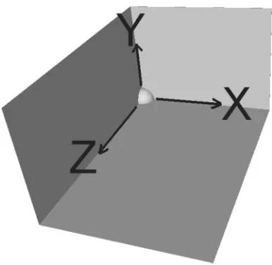
Figure 1: An initialised bin with one corner in the back left bottom corner of the bin.

3

Representation for One-, Two-, and Three-Dimensional

Packing Problems

We will begin the description of our representation by using the example of a 3D knapsack problem. We will then extend the description in Section 3.5 to cover the bin packing problem and to cover problems of lower dimensions.

3.1 Bin and Corner Objects

Each bin is represented by its dimensions and by a list of corner objects, which represent the available spaces into which a piece can be placed. A bin is initialised by creating a corner which represents the lower back left corner of the bin, as shown in Figure 1. Therefore at the start of the packing, the heuristic just chooses which piece to put into this corner, because it is the only one available. Figure 1 also shows the positive directions of thex, y,andzaxes.

When the chosen piece is placed, the corner is deleted, as it is no longer available, and at most three more corners are generated in the x, y,and z directions from the coordinates of the deleted corner. This is shown in Figure 2. A corner is not created when the piece meets the outside edge of the container. Therefore, after the first piece has been put into the bin, the heuristic then has a choice of a maximum of three corners that the first piece defines.

A corner contains information about the three 2D surfaces that intersect to define it, in the xy plane, thexzplane, and theyzplane. The corner is at the intersection of these three orthogonal planes, and the size and limits of the three surfaces are defined by the extent of the piece faces (or container faces) that intersect at the corner. Figure 3 shows the three 2D surfaces that the corner above the piece is defined by. Note that the

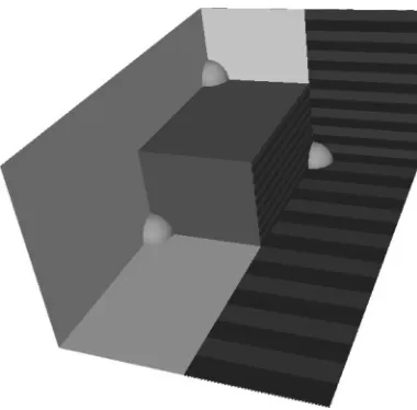
Figure 2: A bin with one piece placed in the corner of Figure 1.

Figure 3: The three surfaces defined by the corner that is in theydirection of the piece.

3.2 Valid Placement of Pieces

Automated Design of Packing Heuristics

Figure 4: The three surfaces defined by the corner that is in thexdirection of the piece.

Figure 5: An invalid placement of a new piece, because it exceeds the limit of the corner’sxzsurface in thezdirection.

3.3 Extending a Corner’s Surfaces

Figure 6: An invalid placement of a new piece, because it exceeds the limit of the corner’syzsurface in thezdirection.

Figure 7: A piece which reaches the limit of two surfaces of the corner that it was put into.

3.4 Filler Pieces

Automated Design of Packing Heuristics

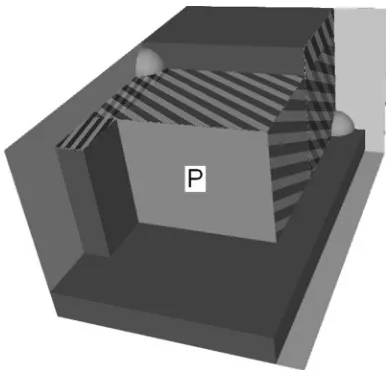
Figure 8: The three surfaces of the corner with the smallest avaliable area.

Figure 9: A filler piece is put into corner A from Figure 8, and the surfaces of two corners are updated.

The reason for the filler piece is that it will exactly reach the edge of an adjacent piece, and extend the surface that it matches with, therefore increasing the number of pieces that will fit into the corner that the surface belongs to. As is shown in Figure 9, three corners have their surfaces updated by the filler piece. First, the corner in the top left of the figure has itsxzsurface extended across the top of the filler piece in the

x direction, shown by horizontal stripes. Secondly, the corner to the left of the filler piece has itsxysurface extended across the front of the piece, shown by vertical stripes. Thirdly, the corner just under the filler piece receives a secondyzsurface, which extends up the right side of the filler piece. Both the originalyzsurface and the second one are shown in the figure as diagonal stripes. Note that a filler piece never creates a corner, thus the net effect of inserting a filler piece will be the deletion of the corner that the filler piece was inserted into.

After the filler piece has been placed, this process is repeated, and if the corner with the next smallest available area cannot accept any remaining piece, then that corner is filled with a filler piece. As soon as the smallest corner can accept at least one piece from those remaining, we continue the packing. In the knapsack problem there is only one bin. The packing will terminate when the whole bin is filled with pieces and filler pieces, so there are no corners left. The result is then the total value of the pieces in the knapsack.

3.5 Bin Packing, and Packing in Lower Dimensions

The representation described in Sections 3.1–3.4 also allows for the bin packing problem to be represented. If the user specifies that the instance is to be used for the bin packing problem, then an empty bin is always kept open so the evolved heuristic can choose to put a piece in it; then if this bin is used, a new one is opened. The heuristic always has the choice of any corner in any bin. When running an instance as a bin packing problem, the piece values are set to one because they are not relevant, and the packing stops when all the pieces have been packed.

The 3D representation can also be used for 1D and 2D problem instances by setting the redundant dimensions of the bins and pieces to one. For example, when using a 2D instance, the depth of each piece and bin is set to one, and for a 1D instance, the depth and height are set to one.

4

The Genetic Programming Methodology

This section describes the evolutionary algorithm that evolves packing heuristics. Each program in the genetic programming population is a packing heuristic, and is applied to a packing problem to obtain a result. The heuristics are then manipulated by the genetic programming system depending on their performance. We will refer to a combination of piece, orientation, and corner as an allocation, and a point in the algorithm where the heuristic is asked to decide which piece is placed where will be referred to as a decision point. Sections 4.1 and 4.2 describe how a heuristic is applied, and Sections 4.3 and 4.4 describe how the population of heuristics are evolved.

4.1 How the Heuristic Is Applied

Automated Design of Packing Heuristics

terminal nodes are set to the values they represent, and the function nodes perform operations on the values returned by their child nodes. More information on functions and terminals can be found in introductory genetic programming references (Koza, 1992; Banzhaf et al., 1998; Koza and Poli, 2005).

The heuristic returns one numerical value each time it is evaluated, which is then interpreted as a score for the allocation. So every piece, orientation, and corner com-bination, in every bin, is evaluated in this way. The actual allocation performed is the one which receives the maximum evaluation (score). Then the filler stage (Section 3.4) is performed to fill any redundant space, and the cycle then repeats at the next decision point. This process is shown in Algorithm 1.

To evaluate a heuristic for a valid allocation, its terminal values are set to values dictated by the properties of the current allocation, that is, the properties of the current piece, orientation, and corner (see Section 4.2 for further clarification of this process). One numerical value is returned by the heuristic, which is interpreted as an evaluation of the relative suitabilility of the allocation.

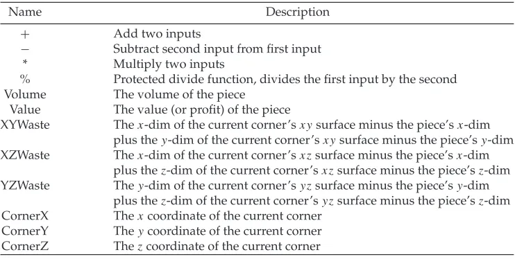
Table 1: The functions and terminals and descriptions of the values they return.

Name Description

+ Add two inputs

− Subtract second input from first input * Multiply two inputs

% Protected divide function, divides the first input by the second Volume The volume of the piece

Value The value (or profit) of the piece

XYWaste Thex-dim of the current corner’sxysurface minus the piece’sx-dim plus they-dim of the current corner’sxysurface minus the piece’sy-dim XZWaste Thex-dim of the current corner’sxzsurface minus the piece’sx-dim

plus thez-dim of the current corner’sxzsurface minus the piece’sz-dim YZWaste They-dim of the current corner’syzsurface minus the piece’sy-dim

plus thez-dim of the current corner’syzsurface minus the piece’sz-dim CornerX Thexcoordinate of the current corner

CornerY Theycoordinate of the current corner CornerZ Thezcoordinate of the current corner

When solving a bin packing problem, the framework always keeps an empty bin available to the heuristic. When solving a knapsack problem, only one bin is available, and this will eventually be filled up (with pieces and filler pieces) so that there are no corners left. When this occurs, the knapsack packing is complete, and the heuristic has been used to form a solution. In summary, the heuristic chooses which piece to pack next, and into which corner, by returning a value for each possible combination. The combination with the highest value is taken as the heuristic’s choice.

4.2 Genetic Programming Functions and Terminals

Table 1 summarises the 12 functions and terminals and the values they return; the functions are shown in the top four rows, and the terminals in the lower eight rows. The arithmetic operators add, subtract, multiply, and protected divide are chosen to be included in the function set. Genetic programming usually uses protected divide instead of the standard divide function because there is always a possibility that the denominator will be zero. The protected divide function replaces a zero denominator by 0.001.

The first two terminals shown in Table 1 represent attributes of the piece. The first terminal represents the volume of the piece. If needed, some kind of piece priority based on size can be evolved because of the information this terminal provides to the heuristic. The second terminal represents the value of the piece. This information is useful only in the knapsack problem, but is still left in the terminal set when a heuristic is being evolved for bin packing, because one of our aims is to demonstrate that the proposed algorithm requires no parameter modification or tuning. Therefore, in the bin packing case, the value terminal will always return one. Both the volume and the value terminals could, for example, be used in the heuristic to prioritise pieces based on their value per unit volume.

The three waste terminals give the heuristic information on how good a fit the piece is to the corner under consideration. There is one for each surface of the corner xy,

Automated Design of Packing Heuristics

Finally, there are three terminals, cornerX, cornerY, and cornerZ, which provide the heuristic with information about the position of the corner in the container. They return the relevant coordinate of the corner. For example, cornerY returns they coordinate of the current corner.

4.3 Fitness of a Heuristic

Each heuristic in the population packs the given instance, and its fitness is assigned to it based on the quality of the packing. The quality of the packing is necessarily calculated differently for bin packing and knapsack instances.

4.3.1 Bin Packing Fitness

For bin packing problems, we use the fitness function shown in Equation (3), based on that presented by Falkenauer and Delchambre (1992), wheren=number of bins,m=

number of pieces.vj =volume of piecej.xij =1 if piecej is in biniand 0 otherwise, andC=bin volume (capacity). Only the bins that contain at least one piece are included in this fitness function.

Fitness=1−

⎛ ⎜ ⎝

n i=1

m j=1vjxij

C 2 n ⎞ ⎟ ⎠ (3)

This fitness function puts a premium on bins that are nearly or completely filled. Importantly, the fitness function avoids the problem of plateaus in the search space, which occur when the fitness function is simply the number of bins used by the heuristic (Burke, Hyde et al., 2006). We subtract from one as the term in brackets equates to values between zero and one and we are interested in minimising the fitness value.

4.3.2 Knapsack Fitness

For knapsack problems, the fitness of a heuristic is the total value of all of the pieces that have been chosen by the heuristic to be packed into the single knapsack. The reciprocal of this figure is then taken to be the fitness because the genetic programming implementation treats lower fitness values as better. This fitness function is shown in Equation (4), wheren represents the number of pieces in the instance,xj is a binary variable indicating if the piecej is packed in the knapsack, andvj represents the value of the piecej.

Fitness= n 1

j₌1vjxj

(4)

4.4 Genetic Programming Parameters

Table 2 shows the parameters used in the genetic programming runs. The mutation operator uses the grow method described by Koza (1992), with a minimum and max-imum depth of five, and the crossover operator produces two new individuals with a maximum depth of 17. These are standard default parameters provided in the genetic programming implementation of the ECJ (Evolutionary Computation in Java) package we used for our experiments.

5

The Datasets

Table 2: Parameters of each genetic programming run.

Population size 1,000

Generations 50

Crossover probability 0.85

Mutation probability 0.1

Reproduction probability 0.05

Tree initialisation method Ramped half-and-half

Selection method Tournament selection, size 7

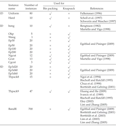
Table 3: A summary of the 18 datasets used in this paper.

Used for Instance Number of

name instances Bin packing Knapsack References

1D Uniform 80 √ × Falkenauer (1996)

Hard 10 √ × Scholl et al. (1997)

Schwerin and Wascher (1997)

2D beng 10 √ × Bengtsson (1982)

Martello and Vigo (1998)

Okp 5 × √

Wang 1 × √

Ep30 20 × √

Egeblad and Pisinger (2009)

Ep50 20 × √

Ep100 20 × √

Ep200 20 × √

Ngcut 12 √ √ Egeblad and Pisinger (2009)

Gcut 13 √ √ Martello and Vigo (1998)

Cgcut 3 √ √

3D Ep3d20 20 × √

Ep3d40 20 × √ Egeblad and Pisinger (2009)

Ep3d60 20 × √

Thpack8 15 × √ Ngoi et al. (1994)

Bischoff and Ratcliff (1995) Chua et al. (1998)

Bortfeldt and Gehring (2001)

Thpack9 47 √ √ Huang and He (2009)

Ivancic et al. (1989) Bischoff and Ratcliff (1995) Eley (2002)

Lim and Zhang (2005)

BandR 700 × √ Egeblad and Pisinger (2009)

Automated Design of Packing Heuristics

Table 4: Summary of bin packing results, and the percentage improvement over the best results in the literature.

Instance name Ratio SD Percent difference

1D Uniform 1.000 0.003 0

Hard 1.004 0.007 −0.4

2D Beng 1.000 0.053 0

Ngcut 1.000 0.000 0

Gcut 1.012 0.041 −1.2

Cgcut 1.000 0.000 0

3D Thpack9 1.023 0.086 −2.3

methodologies. Instances that are originally created as knapsack instances can be used as bin packing instances by ignoring the value of each piece, and packing all the pieces in the instance into the fewest bins possible. Instances originally intended as bin packing problems do not specify a value for each piece, so to use them as knapsack instances it is usual for practitioners to set each piece’s value equal to its volume. The instances are used in a large number of papers. In Table 3 we give the references where the instances have been used to obtain the results we have compared against in this paper. They use the same set of constraints, meaning we can compare fairly with these results.

6

Results

We obtain results on a suite of 18 datasets, the details of which are shown in Section 5. Each dataset contains a number of instances. We compare our results for an instance against the result of the best heuristic in the literature for that instance. Tables 4 and 5 show the Ratio for each dataset, which is a value obtained by comparing our results for a dataset to the best results in the literature. To get to this Ratio figure, there are three steps, described below and shown in Equations (5), (6), and (7).

For every instance, we perform 10 runs, each with a different random seed. We calculate the average over the 10 runs for the instance, and name this value the In-stanceAverage. This is shown in Equation (5), whereriis the result of runi.

For each instance, we then calculate the ratio of the InstanceAverage over the best result in the literature, and name this value the InstanceRatio. This is shown in Equation (6), wherezis the best result in the literature for the given instance.

Each instance in a set has an InstanceRatio, and the Ratio is the average Instance-Ratio of all the instances in the set. This is shown in Equation (7), whereiis the instance number, andmis the number of instances in the data set.

InstanceAverage= 10

i₌1ri

10 (5)

InstanceRatio= InstanceAverage

z (6)

Ratio= m

i=1InstanceRatioi

m (7)

Tables 4 and 5 show the Ratio for each dataset. The standard deviation reported is for the distribution of InstanceRatio values, of which there will be one for every instance in the set.

Table 5: Summary of knapsack results, and the percentage improvement over the best results in the literature.

Instance name Ratio SD Percent difference

2D Okp 1.012 0.019 +1.2

Wang 1.000 0.000 0

Ep30 0.991 0.018 −0.9

Ep50 1.004 0.014 +0.4

Ep100 0.974 0.072 −2.6

Ep200 1.024 0.015 +2.4

Ngcut 0.957 0.143 −4.3

Gcut 1.012 0.062 +1.2

Cgcut 0.983 0.016 −1.7

3D Ep3d20 1.130 0.107 +13.0

Ep3d40 1.102 0.100 +10.2

Ep3d60 1.060 0.067 +6.0

Thpack8 0.995 0.014 −0.5

Thpack9 1.007 0.000 +0.7

BandR 0.971 0.004 −2.9

problem is a maximisation problem, so a Ratio higher than one means our result is better. To keep the results consistent, we convert the Ratios to a percentage value which represents our improvement over the best results in the literature. For example, a Ratio of 1.023 as a bin packing result represents a –2.3% improvement, because it means that, in the results we obtained, we use 2.3% more bins on average. This percentage figure is shown in Tables 4 and 5.

6.1 Bin Packing Results

The discussion in this section refers to the results reported in Table 4.

6.1.1 One Dimensional

For the Uniform dataset, we compare to Falkenauer (1996). Our results are one bin worse than Falkenauer’s results for three instances out of 80. We obtain results one bin better for two instances out of the 80, achieving the proven optimum results in those cases. Also, for each instance, our average of the 10 runs is never more than one bin worse than our best result, so in this respect the results are consistent.

For the Hard dataset, we compare to Schwerin and Wascher (1997), who have solved the instances to optimality. We achieve the optimal result for all but one instance of the set of 10, where our best result uses one bin more than the optimal. For seven of the instances, we find the optimal result in all 10 runs.

6.1.2 Two Dimensional

For the Beng dataset, our results are compared to the exact methods of Bengtsson (1982) and Martello and Vigo (1998). For the Ngcut, Gcut, and Cgcut sets, we compare our results to Martello and Vigo (1998). The results that have been reported for these four datasets are obtained without allowing rotations of the pieces, so for a fair comparison we applied the same constraint.

Automated Design of Packing Heuristics

6.1.3 Three Dimensional

Thpack9 is the only 3D bin packing instance. For 42 instances out of the 47, our best heuristic evolved from the 10 runs matches the best result from the literature. There are four instances in which we use one more bin than the best result, and one instance in which we beat the best result by one bin. The average number of bins used in each of the 10 runs is never more than 0.7 greater than the best result of the 10 runs, so the heuristics evolved are of consistently good quality for each instance.

6.2 Knapsack Results

The discussion in this section refers to the results reported in Table 5.

6.2.1 Two Dimensional

We compare all our 2D knapsack results to the results of Egeblad and Pisinger (2009), who define the four new Ep* instance sets to test their heuristic. They also apply their heuristic approach to five older datasets, previously solved to optimality with exact methods but still useful to compare heuristic methods which are not guaranteed to achieve the optimal result.

Our results on the nine problem sets show that there is no real difference between the performance of our evolved heuristics and the performance of the heuristic method presented by Egeblad and Pisinger (2009). There are five sets with Ratio just greater than one, and four just less than one. In the ngcut set, the high standard deviation is because of the sixth instance of the set where the Ratio is 0.5. Without this outlier the standard deviation of ngcut would be less than 0.01.

6.2.2 Three Dimensional

There are three subsets in the ep3d set. In the first set, with instances of 20 pieces, our results are better in every instance than the results of Egeblad and Pisinger (2009). In the second set our results are better in all but two instances, and in the third set all but four of our results are better.

Thpack8 has 15 instances. In 13 of those, we match the best result for the instance from five papers that report results. However, in the second and sixth instances in the set, our system could not reach the results of the CBUSE method of Bortfeldt and Gehring (2001). However our result for the second instance is only beaten by CBUSE in the literature, and the result for the sixth instance is third best in the literature.

Over the 47 instances of Thpack9, we obtain an average space utilisation of 95.2%, which is compared to the 94.6% of Huang and He (2009). We get 100% space utilisation in 14 instances out of the 47. The individual results for the 47 instances of this set are not reported, so in this dataset we could not use Equations (5), (6) and (7). Therefore, in the Ratio column of Table 5 for this dataset, we report the Ratio of our average space utilisation over the average space utilisation of Huang and He (2009). This also means that the standard deviation is not reported because we could not calculate InstanceRatio values for each instance of this dataset.

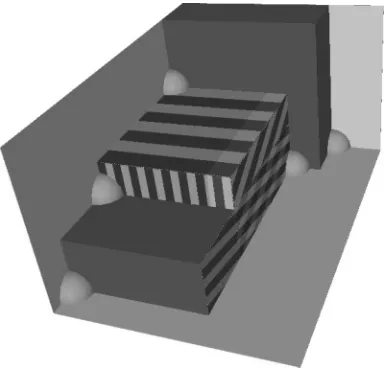
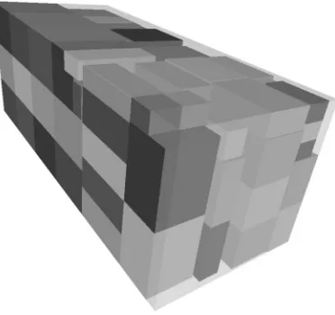
Figure 10: An example heuristic which was evolved on the instance BR5-0, displayed in prefix notation. The terminal names are abbreviated to save space. X, Y, and Z are the corner coordinates, V is the piece value, v is the piece volume, and XZ is the XZWaste terminal.

Figure 11: The solution to instance BR5-0 found by the heuristic in Figure 10.

So for each of the seven subsets, we compile the best average space utilisation reported in the literature from the five papers that report results. We calculate the equivalent of an InstanceRatio for each subset, by dividing our average for the subset by the best result for the subset. Then the Ratio is calculated with Equation (7) withm

set to seven. So for the BandR data set, we are comparing against the best technique on each of its seven subsets, rather than on each instance.

7

An Example Evolved Heuristic

In this section we give an example of an evolved heuristic, which was evolved on the 3D knapsack instance BR5-0. This instance is the first in the set of 100 in the BR5 class, each of which have 12 different sizes of pieces in different quantities. Figure 10 shows the heuristic in prefix notation, and Figures 11 and 12 show the result on the BR5-0 instance from two different angles.

Automated Design of Packing Heuristics

Figure 12: The same solution as Figure 11, viewed from underneath.

Figure 13: The values returned by the example evolved heuristic in Figure 10, when the volume of the piece is changed for three different values of XZWaste. The graph shows that for any given volume of a piece, it will be placed in the orientation that minimises its XZWaste.

highest result from the heuristic. This seems to suggest that when there is a choice of pieces to place into a corner, the largest piece will be chosen. However, the behaviour of the heuristic cannot be described as simply as this, because an increase in the volume of the box will usually result in a reduction in the waste of one or more of the three surfaces at the corner. Therefore, the other terminals cannot realistically be treated as fixed.

Figure 14: The values returned by the example evolved heuristic in Figure 10, when the CornerX, CornerY, and CornerZ terminals change their values. The values are shown when each is set to between 0 and 45, with the other two terminals fixed at 20. The Volume and Value terminals are set to 200,000, and the Waste terminals are fixed at 20. The graph shows that, with all other terminals being equal, a piece will be placed at a smaller x coordinate, and a largery coordinate. The zcoordinate makes very little difference.

20. The graph shows that, in general, an allocation will be considered better if the xz

waste is lower, and this will be the dominating component especially at low values of XZWaste. However, another piece with more waste can be considered better if is at least a certain volume. For example, Figure 13 shows that an allocation with XZWaste=5 and a piece volume of 100,000 will be rated lower than an allocation with XZWaste= 10 (more wasted space) and a piece volume of 350,000 or greater. So there is a volume threshold above which a piece with more XZWaste will be put in ahead of one that fits better onto thexzsurface. The graph also shows that a piece will be placed in the orientation that minimises its XZWaste.

The line for XZWaste=0 is not shown because it is significantly above the scale of they axis in Figure 13. The values returned by the heuristic for a piece which has no XZWaste are on the order of 1014_{, much higher than 10}4 _{which is returned when there}

is an XZWaste of five. If a piece fits exactly onto the XZ surface, then it will always be placed there regardless of the size of the pieces in alternative allocations.

The heuristic will mostly have a choice of more than one corner into which to put a piece. Figure 14 shows the effect of differing values for the CornerX, CornerY, and CornerZ terminals. This graph shows that the value returned by the heuristic decreases when the x coordinate of the corner increases, so the heuristic prefers to put pieces closer to the left side of the container. When theycoordinate of the corner increases, the value returned by the heuristic increases, so it prefers to put pieces into higher corners given the samex andzcoordinate. Thezcoordinate has almost no effect on the value returned by the heuristic.

Automated Design of Packing Heuristics

if there is a choice. This tower building behaviour can be seen to some extent in Figures 11 and 12, where the left side of the container is filled with large identical pieces. The heuristic completes each tower of three pieces before starting the next one in front of it, showing that the heuristic considers the higher piece allocations to be better. More irregular towers can be seen at the front of the solution, where each piece fits well to the piece below.

8

Conclusions

In this paper, we have described a genetic programming methodology that evolves a heuristic for any 1D, 2D, or 3D knapsack or bin packing problem. This methodology can be described as a hyper-heuristic, because it searches a space of heuristics rather than a space of solutions directly. It differs from many of the hyper-heuristic methodologies in the literature because its aim is not to choose from a set of prespecified heuristics, but to automatically generate one heuristic from a set of potential components.

We have presented the results obtained by these automatically designed heuristics, and have shown them to be highly competitive with the state of the art human created heuristics and metaheuristics. Therefore, the contribution of this paper is to show that computer designed heuristics can at least equal the performance of human designed heuristics in the packing problems addressed here. This is especially significant as these packing problems are well studied, and the human created heuristics obtain very close to optimal solutions for some of the datasets.

Automatic heuristic generation is a new area of research. The traditional method of solving packing problems is to obtain or generate a set of benchmark instances, and design a heuristic that obtains good results for that dataset. This process of heuristic design can take a long time, after which the resulting heuristic can be specialised to the benchmark dataset. Recently, metaheuristics have been developed which operate well over large instances, and a variety of instance sets. Designing a metaheuristic system, and optimising its parameters, is a process that can take many more hours of research. Currently, in the cutting and packing literature, systems are developed for one problem domain. For example, a metaheuristic system developed solely for 3D packing instances cannot usually operate on 1D instances. This paper represents the first packing system that can successfully operate over different problem domains. The system can be this general because it can generate new heuristics for each problem domain.

Therefore, in addition to showing that human competitive heuristics can be auto-matically designed, a further contribution of this paper is to present a system that can generate a solution for any 1D, 2D, or 3D knapsack or bin packing problem instance, with no change of parameters in between. All that is required is to provide the problem instance file, and specify whether it is a bin packing or knapsack instance. One of the goals of hyper-heuristic research is to “raise the level of generality” of search methods. We conclude that the methodology presented here represents a more general system than those currently available, due to its performance on problems in the 1D, 2D, and 3D cases of two packing problem domains.

References

Alvarez-Valdes, R., Parreno, F., and Tamarit, J. M. (2009). A branch and bound algorithm for the strip packing problem.Operations Research Spectrum, 31(2):431–459.

Baker, B. S., Coffman, E. G., and Rivest, R. L. (1980). Orthogonal packings in two dimensions.

Banzhaf, W., Nordin, P., Keller, R., and Francone, F. (1998). Genetic programming; An introduction: On the automatic evolution of computer programs and its applications. San Mateo, CA: Morgan Kaufmann.

Beasley, J. E. (1985). An exact two-dimensional non-guillotine cutting tree search procedure.

Operations Research, 33(1):49–64.

Bengtsson, B. E. (1982). Packing rectangular pieces—A heuristic approach.The Computer Journal, 25(3):353–357.

Bischoff, E., and Ratcliff, M. (1995). Issues in the development of approaches to container loading.

Omega, 23(4):377–390.

Bortfeldt, A., and Gehring, H. (2001). A hybrid genetic algorithm for the container loading problem.European Journal of Operations Research, 131(1):143–161.

Bortfeldt, A., Gehring, H., and Mack, D. (2003). A parallel TABU search algorithm for solving the container loading problem. Parallel Computing, 29(5):641–662.

Burke, E., Kendall, G., and Whitwell, G. (2004). A new placement heuristic for the orthogonal stock-cutting problem. Operations Research, 55(4):655–671.

Burke, E., Kendall, G., and Whitwell, G. (2009). A simulated annealing enhancement of the best-fit heuristic for the orthogonal stock cutting problem.INFORMS Journal on Computing, 21(3):505–516.

Burke, E. K., Hart, E., Kendall, G., Newall, J., Ross, P., and Schulenburg, S. (2003). Hyper-heuristics: An emerging direction in modern search technology. In F. Glover and G. Kochenberger (Eds.),Handbook of meta-heuristics(pp. 457–474). Dordrecht, The Netherlands: Kluwer.

Burke, E. K., Hellier, R. S. R., Kendall, G., and Whitwell, G. (2006). A new bottom-left-fill heuristic algorithm for the two-dimensional irregular packing problem.Operations Research, 54(3):587–601.

Burke, E. K., Hyde, M., and Kendall, G. (2010). Providing a memory mechanism to enhance the evolutionary design of heuristics. InProceedings of the IEEE World Congress on Computational Intelligence (WCCI’10), pp. 3883–3890.

Burke, E. K., Hyde, M., Kendall, G., Ochoa, G., ¨Ozcan, E., and Woodward, J. (2009). Exploring hyper-heuristic methodologies with genetic programming. In C. Mumford and L. Jain (Eds.), Computational intelligence: Collaboration, fusion and emergence(pp. 177–201). Berlin: Springer.

Burke, E. K., Hyde, M., Kendall, G., Ochoa, G., Ozcan, E., and Woodward, J. (2010). A classification of hyper-heuristics approaches. In M. Gendreau and J. Potvin (Eds.), Handbook of meta-heuristics,2nd ed. (pp. 449–468). Berlin: Springer.

Burke, E. K., Hyde, M. R., and Kendall, G. (2006). Evolving bin packing heuristics with genetic programming. In T. Runarsson, H.-G. Beyer, E. Burke, J. Merelo-Guervos, D. Whitley, and X. Yao (Eds.),Proceedings of the 9th International Conference on Parallel Problem Solving from Nature (PPSN 2006). Lecture Notes in Computer Science, Vol. 4193 (pp. 860–869). Berlin: Springer-Verlag.

Burke, E. K., Hyde, M. R., Kendall, G., and Woodward, J. (2007a). Automatic heuristic generation with genetic programming: Evolving a jack-of-all-trades or a master of one. InProceedings of the 9th ACM Genetic and Evolutionary Computation Conference (GECCO 2007), pp. 1559–1565.

Automated Design of Packing Heuristics

Burke, E. K., Hyde, M. R., Kendall, G., and Woodward, J. (2010). A genetic programming hyper-heuristic approach for evolving two dimensional strip packing hyper-heuristics.IEEE Transactions on Evolutionary Computation, 14(6):942–958.

Burke, E. K., Kendall, G., and Soubeiga, E. (2003). A tabu-search hyper-heuristic for timetabling and rostering.Journal of Heuristics, 9(6):451–470.

Burke, E. K., Petrovic, S., and Qu, R. (2006). Case-based heuristic selection for timetabling problems.Journal of Scheduling, 9(2):115–132.

Christofides, N., and Whitlock, C. (1977). An algorithm for two-dimensional cutting problems.

Operations Research, 25(1):30–44.

Chua, C. K., Narayanan, V., and Loh, J. (1998). Constraint-based spatial representation technique for the container packing problem.Integrated Manufacturing Systems, 9(1):23–33.

Clautiaux, F., Jouglet, A., Carlier, J., and Moukrim, A. (2008). A new constraint programming approach for the orthogonal packing problem.Computers and Operations Research, 35(3):944– 959.

Coffman, E. G., Jr., Courcoubetis, C., Garey, M., Johnson, D. S., Shor, P. W., Weber, R. R., and Yannakakis, M. (2000). Bin packing with discrete item sizes, Part I: Perfect packing theorems and the average case behavior of optimal packings. SIAM Journal on Discrete Mathematics, 13:384–402.

Coffman, E. G., Jr., Galambos, G., Martello, S., and Vigo, D. (1998). Bin packing approximation algorithms: Combinatorial analysis. In D. Z. Du and P. M. Pardalos (Eds.), Handbook of combinatorial optimization. Dordrecht, The Netherlands: Kluwer.

Cuesta-Canada, A., Garrido, L., and Terashima-Marin, H. (2005). Building hyper-heuristics through ant colony optimization for the 2D bin packing problem. InProceeding of the 9th International Conference on Knowledge-Based Intelligent Information and Engineering Systems (KES’05). Lecture Notes in Computer Science, Vol. 3684 (pp. 654–660). Berlin: Springer-Verlag.

Dowsland, K., Soubeiga, E., and Burke, E. K. (2007). A simulated annealing hyper-heuristic for determining shipper sizes.European Journal of Operations Research,179(3):759–774.

Egeblad, J., and Pisinger, D. (2009). Heuristic approaches for the two- and three-dimensional knapsack packing problem.Computational and Operations Research, 36(4):1026–1049.

Eley, M. (2002). Solving container loading problems by block arrangement. European Journal of Operations Research, 141(2):393–409.

Falkenauer, E. (1996). A hybrid grouping genetic algorithm for bin packing. Journal of Heuristics, 2:5–30.

Falkenauer, E., and Delchambre, A. (1992). A genetic algorithm for bin packing and line balancing. InProceedings of the IEEE 1992 International Conference on Robotics and Automation, pp. 1186– 1192.

Fukunaga, A. S. (2002). Automated discovery of composite SAT variable-selection heuristics. In

Proceedings of Eighteenth National Conference on Artificial Intelligence, pp. 641–648.

Fukunaga, A. S. (2004). Evolving local search heuristics for SAT using genetic programming. In K. Deb et al. (Ed.), Proceedings of the ACM Genetic and Evolutionary Computation Con-ference (GECCO ’04). Lecture Notes in Computer Science, Vol. 3103 (pp. 483–494). Berlin: Springer-Verlag.

Fukunaga, A. S. (2008). Automated discovery of local search heuristics for satisfiability testing.

Geiger, C. D., Uzsoy, R., and Aytug, H. (2006). Rapid modeling and discovery of priority dispatching rules: An autonomous learning approach.Journal of Scheduling, 9(1):7–34.

Gilmore, P., and Gomory, R. (1961). A linear programming approach to the cutting-stock problem.Operations Research, 9(6):849–859.

Hadjiconstantinou, E., and Iori, M. (2007). A hybrid genetic algorithm for the two-dimensional sin-gle large object placement problem.European Journal of Operations Research, 183(3):1150–1166.

Hopper, E., and Turton, B. C. H. (2001). An empirical investigation of meta-heuristic and heuristic algorithms for a 2D packing problem.European Journal of Operations Research, 128(1):34–57.

Huang, W., and He, K. (2009). A new heuristic algorithm for cuboids packing with no orientation constraints. Computers and Operations Research, 36(2):425–432.

Hwang, S. M., Kao, C. Y., and Horng, J. T. (1994). On solving rectangle bin packing problems using genetic algorithms. InProceedings of the 1994 IEEE International Conference on Systems, Man, and Cybernetics, Vol. 2, pp. 1583–1590.

Ivancic, N., Mathur, K., and Mohanty, B. (1989). An integer-programming based heuristic approach to the three-dimensional packing problem.Journal of Manufacturing and Operations Management, 2:268–298.

Johnson, D., Demers, A., Ullman, J., Garey, M., and Graham, R. (1974). Worst-case performance bounds for simple one-dimensional packaging algorithms. SIAM Journal on Computing, 3(4):299–325.

Keller, R. E., and Poli, R. (2007). Linear genetic programming of parsimonious metaheuristics. InProceedings of the IEEE Congress on Evolutionary Computation (CEC 2007), pp. 4508–4515.

Kenmochi, M., Imamichi, T., Nonobe, K., Yagiura, M., and Nagamochi, H. (2009). Exact algorithms for the two-dimensional strip packing problem with and without rotations.

European Journal of Operational Research, 198(1):73–83.

Kenyon, C. (1996). Best-fit bin-packing with random order. InProceedings of the Seventh Annual ACM-SIAM Symposium on Discrete Algorithms, pp. 359–364.

Koza, J. R. (1992). Genetic programming: On the programming of computers by means of natural selection. Cambridge, MA: MIT Press.

Koza, J. R., and Poli, R. (2005). Genetic programming. In E. K. Burke and G. Kendall (Eds.),

Search methodologies: Introductory tutorials in optimization and decision support techniques(pp. 127–164). Dordrecht, The Netherlands: Kluwer.

Lagus, K., Karanta, I., and Yla-Jaaski, J. (1996). Paginating the generalized newspaper, A comparison of simulated annealing and a heuristic method. In Proceedings of the 5th International Conference on Parallel Problem Solving from Nature (PPSN ’96), pp. 549–603.

Lim, A., Rodrigues, B., and Wang, Y. (2003). A multi-faced buildup algorithm for three-dimensional packing problems. OMEGA International Journal of Management Science, 31(6):471–481.

Lim, A., and Zhang, X. (2005). The container loading problem. InProceedings of the 2005 ACM Symposium on Applied Computing (SAC’05), pp. 913–917.

Macedo, R., Alves, C., and Valerio de Carvalho, J. M. (2010). Arc-flow model for the two-dimensional guillotine cutting stock problem. Computers and Operations Research, 37(6):991–1001.

Automated Design of Packing Heuristics

Martello, S., and Vigo, D. (1998). Exact solution of the two-dimensional finite bin packing problem.Management Science, 44(3):388–399.

Ngoi, B. K. A., Tay, M. L., and Chua, E. S. (1994). Applying spatial representation techniques to the container packing problem.International Journal of Production Research, 32(1):111–123.

O’Neill, M., Cleary, R., and Nikolov, N. (2004). Solving knapsack problems with attribute grammars. InProceedings of the Third Grammatical Evolution Workshop (GEWS’04).

Rhee, W. T., and Talagrand, M. (1993). On line bin packing with items of random size.Mathematics Operations Research, 18:438–445.

Richey, M. B. (1991). Improved bounds for harmonic-based bin packing algorithms. Discrete Applied Mathematics, 34:203–227.

Ross, P. (2005). Hyper-heuristics. In E. K. Burke and G. Kendall (Eds.),Search methodologies: Introductory tutorials in optimization and decision support techniques(pp. 529–556). Dordrecht, The Netherlands: Kluwer.

Ross, P., Marin-Blazquez, J. G., Schulenburg, S., and Hart, E. (2003). Learning a procedure that can solve hard bin-packing problems: A new GA-based approach to hyperheurstics. In Proceed-ings of the Genetic and Evolutionary Computation Conference 2003 (GECCO ’03), pp. 1295–1306.

Ross, P., Schulenburg, S., Marin-Blazquez, J. G., and Hart, E. (2002). Hyper heuristics: Learning to combine simple heuristics in bin packing problems. In Proceedings of the Genetic and Evolutionary Computation Conference 2002 (GECCO ’02).

Schneider, W. (1988). Trim-loss minimization in a crepe-rubber mill; Optimal solution versus heuristic in the 2 (3)-dimensional case.European Journal of Operations Research, 34(3):249–412.

Scholl, A., Klein, R., and Jurgens, C. (1997). Bison: A fast hybrid procedure for exactly solving the one-dimensional bin packing problem.Computer and Operations Research, 24(7):627–645.

Schwerin, P., and Wascher, G. (1997). The bin-packing problem: A problem generator and some numerical experiments with FFD packing and MTP. International Transactions in Operations Research, 4(5):377–389.

Seiden, S., Van Stee, R., and Epstein, L. (2003). New bounds for variable-sized online bin packing.

SIAM Journal on Computing, 32(2):455–469.

Terashima-Marin, H., Flores-Alvarez, E. J., and Ross, P. (2005). Hyper-heuristics and classifier systems for solving 2D-regular cutting stock problems. InProceeedings of the ACM Genetic and Evolutionary Computation Conference (GECCO’05), pp. 637–643.

Terashima-Marin, H., Ross, P., Farias-Zarate, C. J., Lopez-Camacho, and Valenzuela-Rendon (2008). Generalized hyper-heuristics for solving 2D regular and irregular packing problems.

Annals of Operations Research, 1(10): 1–10.

Terashima-Marin, H., Zarate, C. J. F., Ross, P., and Valenzuela-Rendon, M. (2006). A GA-based method to produce generalized hyper-heuristics for the 2D-regular cutting stock problem. In

Proceedings of the Genetic and Evolutionary Computation Conference (GECCO’06), pp. 591–598.

Terashima-Marin, H., Zarate, C. J. F., Ross, P., and Valenzuela-Rendon, M. (2007). Comparing two models to generate hyper-heuristics for the 2D-regular bin-packing problem. InProceedings of the Genetic and Evolutionary Computation Conference (GECCO’07), pp. 2182–2189.

Vasko, F. J., Wolf, F. E., and Stott, K. L. (1989). A practical solution to a fuzzy two-dimensional cutting stock problem.Fuzzy Sets and Systems, 29(3):259–275.

Yao, A. C.-C. (1980). New algorithms for bin packing. Journal of the ACM, 27(2):207–227.