Comparing System Dynamics and Agent-Based Simulation for Tumour Growth
and its Interactions with Effector Cells
Grazziela P. Figueredo, Uwe Aickelin
IMA Research Group, Computer Science School, Nottingham University, Wollaton Road, Nottingham, NG8 1BB UK [email protected], [email protected]
Keywords: system dynamics simulation, agent-based sim-ulation, immune system simsim-ulation, comparison of system dynamics and agent-based simulation.
Abstract
There is little research concerning comparisons and com-bination of System Dynamics Simulation (SDS) and Agent Based Simulation (ABS). ABS is a paradigm used in many levels of abstraction, including those levels covered by SDS. We believe that the establishment of frameworks for the choice between these two simulation approaches would con-tribute to the simulation research. Hence, our work aims for the establishment of directions for the choice between SDS and ABS approaches for immune system-related problems. Previously, we compared the use of ABS and SDS for mod-elling agents’ behaviour in an environment with no movement or interactions between these agents. We concluded that for these types of agents it is preferable to use SDS, as it takes up less computational resources and produces the same results as those obtained by the ABS model. In order to move this research forward, our next research question is: if we intro-duce interactions between these agents will SDS still be the most appropriate paradigm to be used? To answer this ques-tion for immune system simulaques-tion problems, we will use, as case studies, models involving interactions between tumour cells and immune effector cells. Experiments show that there are cases where SDS and ABS can not be used interchange-ably, and therefore, their comparison is not straightforward.
1.
INTRODUCTION
The current scenario in the simulation field presents paradigms that allow us to build simulation models for var-ious domains. Some of the important simulation approaches are System Dynamics Simulation (SDS), Agent-Based Simu-lation (ABS), Discrete Event SimuSimu-lation (DES) and Dynamic Systems (DS)[3]. New research also combines these meth-ods and defines frameworks for the usage of each paradigm. There is already work comparing SDS/DES, DES/ABS as well as their combinations. However, there is few research on the comparison and combination of SDS and ABS [8]. Hence, our research aims at establishing a framework for the development of simulations involving the choice between
SDS and ABS approaches and their combination for immune system-related problems .
ABS is a paradigm used in many levels of abstraction, in-cluding those levels covered by SDS. As there is this inter-section, some range of simulation problems can be solved by either SDS or ABS. In previous work [1], we compared the use of ABS and SDS for modelling static agents’ behaviour in an immune system ageing problem. By static we mean that there is no movement or interactions between the agents. We concluded that for these types of agents, it is preferable to use SDS instead of ABS. When contrasting the results of both simulation approaches, we see that SDS is less complex and takes up less computational resources, producing the same re-sults as those obtained by the ABS model.
To advance this study, our next inquiring is: Once we have established that SDS is more suitable for static agents than ABS, if we introduce interactions between these agents will SDS still be the most appropriate paradigm to be used?
To answer this question for immune system simulation problems, we use models as case studies, which include in-teractions between tumour cells and immune effector cells. Effector cells are responsible for eliminating tumour cells in the organism. Our goal is to determine which scenarios for immune system simulations inside the SDS/ABS intersection would benefit from SDS resources and those that are more suitable for ABS.
For SDS we need to establish mathematical equations that determine the flows. Therefore we use the models reviewed in [4]. The authors of this study explored existing spatially homogeneous mechanistic mathematical models describing the interactions between a malignant tumor and the immune system. They begin with the simplest (single equation) mod-els for tumor growth and proceed to consider greater im-munological detail (and correspondingly more equations) in steps. For our simulation, we intend to build SDS and ABS for two of the most important mathematical models described in [4]. We intend to use the mathematical model also as ba-sis for the ABS. The idea is to check if the results would be similar and if we can use SDS and ABS for our case studies interchangeably.
Section 4 we draw the conclusions and present future work.
2.
RELATED WORK
The theoretical work presented by [3] compares ABS and SD conceptually, and discusses the potential synergy between them in order to solve problems of teaching decision-making processes. The authors explore the conceptual frameworks for ABS and SD to model group learning. They show the con-ceptual differences between these two paradigms and propose their use in a complementary way. They outstand the lack of knowledge in multi-paradigm simulation involving SD and ABS.
In [6] and [8], the authors present a cross-study of SD and ABS. They define their features and characteristics and con-trast the two methods. Moreover, they also present ideas of how to integrate both approaches. As a continuation of this work, in [7] they present an approach to integrate the SD and ABS techniques for supply chain management problems. They present some preliminary results, which were not the same as the SD simulation alone. Therefore, they propose new tests as future work. In their case study, they were not able to reach the same results with both simulations.
In [9], the authors show the application of both SD and ABS to simulate non-equilibrium ligand-receptor dynamics over a broad range of concentrations. They concluded that both approaches are powerful tools and are also complemen-tary. In their case study, they did not indicate a preferred paradigm, although intuitively SD is an obvious choice when studying systems at a high level of aggregation and abstrac-tion. On the other hand, SD is not capable of simulating re-ceptors and molecules and their individual interactions, which can be done with ABS.
Rahmandad and Sterman [5] compare the dynamics of a stochastic ABS model with those of the analogous determin-istic compartment differential equation model for contagious disease spread. The authors convert the ABS into a differ-ential equation model and examine the impact of individual heterogeneity and different network topologies. The deter-ministic model yields a single trajectory for each parameter set, while stochastic models yield a distribution of outcomes. Moreover, the differential equation model and ABS dynam-ics differ for several metrdynam-ics relevant to public health. The re-sponse of the models to policies can also differ when the base case behaviour is similar. Under some conditions, however, the differences in means are small, compared to variability caused by stochastic events, parameter uncertainty and model boundary.
In our previous work [1], we compared SDS and ABS for a naive T cell output model. In that study, we concluded that for that case study SDS is more suitable. We had a scenario where the agents had no interactions and SDS and ABS produced similar outputs. Therefore, we decided that, in this case, it is
preferable to choose the SDS, as it takes up less computa-tional resources. In order to continue the investigation, which compares these two simulation approaches, we will add inter-actions between agents and compare the results. The descrip-tion of the problem, as well as the mathematical equadescrip-tions can be seen in the next section.
3.
MATHEMATICAL MODELS
In this section, we present mathematical models used as basis for our simulations. The simplest ones involve only one equation and defines mathematical rules for tumour growth (Section 3.1.). The second mathematical model addresses the interactions between tumour cells and immune effector cells. This is shown in Section 3.2..
3.1.
One-Equation Models: Tumour Growth
In this section, we present the simplest mathematical mod-els. They have only one equation that describes how tumours grow. There are three models of tumour growth from [4] con-sidered in this study: the logistic model, the von Bertalanffy model and the Gompertz model.
According to [4], the most general equation describing the dynamics of tumor growth can be written as:
dT
dt =T f(T), (1)
where:
• T is the tumour cell population at time t,
• T(0)>0,
• f(T) specifies the density dependence in proliferation and death of the tumour cells. The density dependence factor can be written as:
f(T) =p(T)−d(T), (2)
where:
• p(T)defines tumour cells proliferation,
• d(T)define tumour cells death.
The expressions for p(T)and d(T)are generally defined by power laws:
p(T) =aTα, (3)
d(T) =bTβ, (4)
Logistic Model: α=0 and β=1 (a,b>0 and b<a for
growth),
von Bertalanffy Model: α=−31andβ=0 (a,b>0 and b<
a for growth),
Gompertz Model: p(T) =a and d(x) =b ln(T) (a,b>0 and eb>a for growth).
3.1.1. SDS for the One-Equation Model
[image:3.612.68.285.230.271.2]We have implemented the one-equation models using SDS. Figure 1 shows the stock and flow diagram used for modelling the mathematical equations. From the SDS perspective, the amount of tumour cells is a stock that will be modified by proliferation and death flows.
Figure 1. SDS diagram for the general one-equation mathe-matical model.
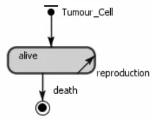
[image:3.612.121.230.369.454.2]3.1.2. ABS for the One-Equation Model
Figure 2. One equation agent.
We have also implemented the one-equation model using ABS. In this case we have a tumour cell agent that will repro-duce and die, as it can be seen in Figure 2.
3.1.3. Experiments
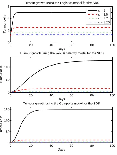
We carried out two experiments to compare the SDS and ABS simulation outputs. For the first experiment, we have established a variable c, which represents the ratio between a and b. The purpose of c is to observe the impact of a and b on the tumour growth curve. Therefore, we set c as 5, 2.5, 1.7 and 1.25.
In the second experiment, we defined a=1.636 and b∈ {0.002,0.005}. These values were determined in [2] and they
will be used for our next simulation set of experiments using a two-equation model.
As the outcomes for ABS are stochastic, we ran each sim-ulation for 50 times and the mean simsim-ulation output is pre-sented. For both simulations, we defined the initial values for tumour cells equal to 1.
3.1.4. Results
For the first experiment, as is shown in Figure 3 (middle and bottom), the outputs for both simulation approaches are similar for the von Bertalanffy and Gompertz models. For the logistics model, on the other hand, the results of the ABS did not match the SDS ones (Figure 3 top). This can be explained by the stochastic and individual behaviour of the agents in the ABS model.
In the experiments, there are few agents on the logistics model and most of them die before they reproduce. In this ABS model, the reproduction rate is given by p(T) =a,
be-cause al pha=0 for the logistics model. In the case where
a=1 and b=0.2, for example, when the number of agents becomes bigger than 5, d(T)gets greater than p(T). As for ABS the death rate is defined for the agents individually, all the newborn tumour cells after 5 agents in the system will have death rates bigger than reproduction rates. Hence, the agents population disappears over the first days. This differ-ence on the SDS and ABS results lead us to conclude that there are cases using static agents where SDS and ABS out-puts will not be the same.
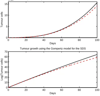
Nevertheless, if we increase the difference between the pa-rameters a and b, as is shown in Figure 4, we avoid the pre-mature death of the tumour agents and therefore the ABS and SDS results become similar again. From what we have found on the literature, the Logistics model is one of the most used for average tumours whereas the von Bertalanffy and Gom-pertz models are used for more aggressive tumours. There-fore, as we increase in the difference between a and b, the Gompertz and von Bertalanffy models growth will present a considerable increase on the proliferation of tumour cells, as illustrates Figure 5.
Therefore, we could not carry out experiment two using ABS for Gompertz and von Bertalanffy models. From the SDS results, we can see that the number of tumour cells by-passes the magnitude of 1064 in the Gompertz model
0 20 40 60 80 100 0
2 4 6
Tumour cells
Days
Tumour growth using the Logistics model for the SDS
0 20 40 60 80 100
0 50 100
Tumour cells
Days
Tumour growth using the von Bertalanffy model for the SDS
0 20 40 60 80 100
0 50 100 150
Tumour cells
Days
Tumour growth using the Gompertz model for the SDS
0 20 40 60 80 100
0 2 4 6
Tumour cells
Days
Tumour growth using the Logistics model for the ABS
0 20 40 60 80 100
0 50 100
Tumour cells
Days
Tumour growth using the von Bertalanffy model for the ABS
0 20 40 60 80 100
0 50 100 150
Tumour cells
Days
Tumour growth using the Gompertz model for the ABS c = 5
[image:4.612.103.299.34.293.2]c = 2.5 c = 1.7 c = 1.25
Figure 3. Results for the one-equation model using SDS and ABS.
0 10 20 30 40 50 60 70 80 90 100
0 200 400 600 800
Tumour cells
Days
Tumour growth using the Logistics model for the SDS
a = 1.636, b = 0.002 a = 1.636, b = 0.004
0 10 20 30 40 50 60 70 80 90 100
0 200 400 600 800
Tumour cells
Days
[image:4.612.104.520.34.425.2]Tumour growth using the Logistics model for the ABS
Figure 4. Results for the second experiment of one-equation Logistics model using SDS and ABS.
3.2.
Two-Equation Models: Interaction
Be-tween Tumour Cells and Generic Effector
Cells
To add complexity to our model, we are going to consider tumour cells growth together with their interactions with gen-eral immune effector cells. In this stage we are not yet con-sidering specific types of immune cells. Effector cells are re-sponsible for killing the tumour cells. They proliferate and die per apoptosis, which is a programmed cellular death. In the models, cancer treatment is also considered.
The interactions between tumour cells and immune effec-tor cells can be defined by the equations:
dT
dt =T f(T)−dT(T,E) (5)
dE
dt =pE(T,E)−dE(T,E)−aE(E) +Φ(T), (6)
where:
• T is the number of tumour cells,
• E is the number of effector cells,
• f(T)is the growth of tumour cells,
• dT(T,E)is the number of tumour cells killed by effector cells,
• pE(T,E)is the proliferation of effector cells,
0 20 40 60 80 100 0
5 10 15
x 104
Tumour cells
Days
Tumour growth using the von Bertalanffy model for the SDS
0 20 40 60 80 100
0 10 20 30 40 50 60 70
Log(Tumour cells)
Days
[image:5.612.357.517.23.86.2]Tumour growth using the Gompertz model for the SDS
Figure 5. Results for the second experiment of one-equation Gompertz and Von Bertalanffy models using SDS.
• Φ(T)is the treatment or influx of cells.
For our models, we used the Kuznetsov model [2]:
f(T) =a(1−bT), (7)
dT(T,E) =nT E, (8)
pE(E,T) = pT E
g+T, (9)
dE(E,T) =mT E, (10)
aE(E) =dE, (11)
Φ(t) =s. (12)
As it can be seen, the Logistic model was adopted for mour growth. It seems to be the most common model of tu-mour growth used in the mathematical models involving can-cer and the immune system. The values for the parameters on the equations can be seen in Table 1. We got these values from [4]. In the first three scenarios we consider cancer treatment. The fourth case does not consider any treatment.
3.2.1. SDS for the Two-Equation Model
We have converted the mathematical model into a SDS model. Figure 6 shows the stock and flow diagram we have defined.
We consider two stocks, the tumour cells and the immune effector cells. The tumour cell stock is changed by prolifera-tion and natural death (as defined in the one-equaprolifera-tion model in Section 2.1); and death caused by the immune effector
Scenario b d s
1 0.002 0.1908 0.318
2 0.004 2 0.318
3 0.002 0.3743 0.1181
4 0.002 0.3743 0
Table 1. Simulation parameters for different scenarios. For the other parameters, the values are the same in all experi-ments, i.e, a=1.636, g=20.19, m=0.00311 ,n=1 and
p=1.131.
[image:5.612.94.255.32.186.2]cells. The immune cells stock is changed by death, apopto-sis, proliferation and injection of new cells as treatment. The number of tumour cells in the organism also stimulates the proliferation of immune cells.
Figure 6. SDS diagram for the two-equation mathematical model.
3.2.2. ABS for the Two-Equation Model
For the ABS model, we defined two agents that will in-teract with each other: the tumour cell agent and the effector cell agent. Figure 7 shows the state charts for the effector cells and the tumour cells. The state chart for the effector cells (left hand side of Figure 7) has two states. Either the cell is alive and able to reproduce or is dead. Effector cells can die by nat-ural means or by damage. The tumour cells state chart also has two states. Tumour cells can reproduce, die with age or die killed by effector cells. The rates defined in the transitions are the same of the mathematical model.
3.2.3. Experiments
As we mentioned before, we carried out four experiments for the two-equation model. The parameter variation for the experiments is shown in Table 1. In the four scenarios, it is considered differences in the death rate of tumour cells fined by the parameter b), effector cells apoptosis rate (de-fined by the parameter d) and treatment (parameter s).
[image:5.612.318.550.227.336.2]Figure 7. ABS diagram for the two-equation mathematical model. On the left hand side we have the state chart for the effector cell agents and on the right hand side we have the state chart for the tumour cell agents.
for the ABS 50 times and display the mean values as the re-sults.
3.2.4. Results
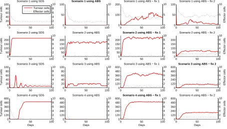
The results comparing SDS and ABS for the four experi-ments can be seen in Figure 8 (first and second columns).
For the first scenario, the behaviour of the tumour cells is very similar for the SDS and ABS results. However, when we ran the Wilcoxon test for the tumour cells outcome, it re-jected the similarity hypothesis for both outcomes, as shown in Table 2. This might be due to the fact that the tumour cells for the SDS model decrease in an asymptotic way to-wards to zero, while ABS behaviour is discrete and hence, it reaches zero. The number of effector cells for both simula-tions follows the same pattern, although the numbers are not the same. The variances in the ABS curve were expected due to its stochastic character.
The results for the second scenario seem to be similar for effector cells, although the Wilcoxon test rejects this hypoth-esis. The results for the tumour cells are not the same.
For scenarios 3 and 4, the results are completely differ-ent for both simulation approaches. Moreover, when we look at the tumour cells curve, the differences are even more evi-dent. In scenario 3 using SDS, tumour cells decrease as effec-tor cells increase, following a predaeffec-tor-prey trend curve. This output is what would be expected by the mathematical model. On the other hand, for the ABS, the number of effector cells decreases until a value close to zero while the tumour cells numbers vary in time differently from the SDS results. The predator-prey behaviour is not observed in this experiment.
In scenario 4, although effector cells seem to decay in a similar trend for both approaches, the results for tumour cells are completely different. In the SDS simulation, the num-bers of tumour cells reach a value close to zero after twenty days and then increases again. For the ABS simulation, on the other hand, tumour cells reach zero and never increase again. It happens because SDS deals with continuous stocks and ABS has a discrete number of agents.
The results in these experiments show that there are
sim-ulation cases where SDS and ABS derived from the same mathematical model do not have the same output. Therefore, it is not possible to compare which approach would be more suitable for these cases.
One alternative would be the development of an ABS so-lution, which is not based on the rates defined in the math-ematical model. However, it seems that for each output (or parameter change on the mathematical model), there should be a different ABS implementation.
For example, if we determine that the number of tumour cells should always be bigger than zero in the ABS, for the second and fourth scenarios the outputs become closer to the SDS, as shown in Figure 8. On the other hand, this constraint also changes the first scenario results, which seemed satisfac-tory before. For scenario 4, although the outcome with this fix do not seem very similar on the beginning of the simulation, the steady state has closer values.
To achieve similar results for scenario 3, we also had to determine that the number of effector cells should be bigger than zero. The results are shown in line 4 of Figure 8. For scenario 3 the fix did not work perfectly. It seems that only the steady state of the simulation has closer results. We also tried to randomly add some effector cells over time, but the results did not looked similar as well.
4.
CONCLUSIONS
The current scenario in the simulation field presents paradigms that allow us to build simulation models for var-ious domains. New research compares simulation methods and defines frameworks for the usage of each paradigm. How-ever, there is few research on the comparison and combina-tion of SDS and ABS [8]. We aim at contributing to this area by studying immune system simulation problems. Therefore, in this study, we used case studies which include interactions between tumour cells and immune effector cells. Our goal was to determine which scenarios for immune system simu-lations inside the SDS/ABS intersection would benefit from SDS resources and those that are more suitable for ABS.
The models we used were reviewed in [4]. We began with the simplest (single equation) models for tumor growth and proceed to consider tow-equation models involving effector and tumour cells. We used mathematical models as basis for both ABS and SDS. The idea was to check if the results would be similar and if we can use SDS and ABS for our case studies interchangeably.
We carried out two experiments to compare the outputs for the one-equation model. For the first experiment, the out-puts for both simulation approaches are similar for two cases. There was an example, though, where the results of the ABS did not match the SDS’s. This is explained by the stochastic and individual behaviour of the agents in the ABS model.
Implementation Cells Scenario
1 2 3 4
p h p h p h p h
ABS Tumour 0 1 0 1 0 1 0 1
Effector 0.0028 1 0.0325 1 0 1 0 1
ABS - Fix 1 Tumour 0 1 0.0103 1 0 1 0.8595 0
Effector 0 1 0.4441 1 0 1 0 1
ABS - Fix 2 Tumour 0 1 0 1 0 1 0 1
[image:7.612.139.473.26.131.2]Effector 0 1 0 1 0 1 0 1
Table 2. Wilcoxon test for tumour cells and effector cells. Comparing the results between SDS and ABS.
0 50 100
0 20 40 60 80 100 Tumour cells
Scenario 1 using SDS
0 50 100
0 50 100 150 200 Tumour cells
Scenario 2 using SDS
0 50 100
0 20 40 60 80 100 Tumour cells
Scenario 3 using SDS
0 50 100
0 120 240 360 480 600 Tumour cells Days Scenario 4 using SDS
0 50 100
0 50 100
Scenario 1 using ABS
0 50 100
0 50 100 150 200
Scenario 2 using ABS
0 50 100
0 20 40 60 80 100
Scenario 3 using ABS
0 50 100
0 120 240 360 480 600 Days Scenario 4 using ABS
0 50 100
0 100 200
Scenario 1 using ABS − fix 1
0 50 100
0 50 100 150 200
Scenario 2 using ABS − fix 1
0 50 100
0 120 240 360 480 600
Scenario 3 using ABS − fix 1
0 50 100
0 120 240 360 480 600 Days Scenario 4 using ABS − fix 1
0 50 100
0 50 100
Scenario 1 using ABS − fix 2
0 50 100
0 50 100 150 200
Scenario 2 using ABS − fix 2
0 50 100
0 120 240 360 480 600
Scenario 3 using ABS − fix 2
0 50 100
0 120 240 360 480 600 Days Scenario 4 using ABS − fix 2
0 50 1000
2 4 6 8 10 Tumour cells Effector cells
0 50 1000
2 4 6 8 10
0 50 1000
2 4 6 8 10
0 50 1000
2 4 6 8 10
0 50 1000
5 10
0 50 1000
2 4 6 8 10
0 50 1000
2 4 6 8 10
0 50 1000
2 4 6 8 10
0 50 1000
5 10
0 50 1000
2 4 6 8 10
0 50 1000
2 4 6 8 10
0 50 1000
2 4 6 8 10
0 50 1000
5 10
Effector cells
0 50 1000
2 4 6 8 10 Effector cells
0 50 1000
2 4 6 8 10 Effector cells
0 50 1000
2 4 6 8 10 Effector cells
Figure 8. Results for the two-equation mathematical model using SDS and ABS. On the first columns we have the SDS results for the four scenarios. The second column has the ABS results. The third and fourth columns shows the fixes we tried to make the outcomes similar. Fix 1 adds the constraint tumour cells>0. Fix 2 adds the constraint tumour cells>0 and e f f ector
cells>0. For each graph we have the results for tumour cells (continuous line) and effector cells (dotted lines). The scale for the tumour cells results is on the left y axis of each graph while the scale for effector cells is in the right y axis.
growth together with their interactions with general immune effector cells. We defined four scenarios and, for only one of them, the results were similar using the mathematical model. The differences in the output are due to the fact that effector cells numbers change continuously on the SDS, while for the ABS, they change in a discrete pattern.
The results in these experiments show that there are sim-ulation cases where SDS and ABS derived from the same mathematical model do not have the same output. Therefore, it is not possible to compare which approach would be more
suitable for these cases.
One alternative would be the development of an ABS so-lution, which is not based on the rates defined in the math-ematical model. However, it seems that for each output (or parameter change on the mathematical model), there should be a different ABS implementation.
[image:7.612.105.559.171.429.2]REFERENCES
[1] Grazziela P. Figueredo and Uwe Aickelin. Investigating im-mune system aging: System dynamics and agent-based mod-elling. In Proceedings of the Summer Computer Simulation
Conference 2010, 2010.
[2] Vladimir A. Kuznetsov, Iliya A. Makalkin, Mark A. Taylor, and Alan S. Perelson. Nonlinear dynamics of immunogenic tumors: parameter estimation and global bifurcation analysis. Bulletin
of Mathematical Biology, 56(2):295–321, 1994.
[3] John Pourdehnad, Kambiz Maani, and Habib Sedehi. System dynamics and intelligent agent based simulation: where is the synergy? In Proceedings of the XX International Conference of
the System Dynamics society., 2002.
[4] D J Earn R Eftimie, J L Bramson. Interactions between the immune system and cancer: A brief review of non-spatial math-ematical models. Bull Math Biol., march 2010.
[5] Hazhir Ramandad and John Sterman. Heterogeneity and net-work structure in the dynamics of diffusion: Comparing agent-based and differential equation models. Management Science, 5(5), may 2008.
[6] Nadine Schieritz. Integrating system dynamics and agent-based modeling. In Proceedings of the XX International Conference
of the System Dynamics society., 2002.
[7] Nadine Schieritz and Andreas Gr¨oßler. Emergent structures in supply chains: a study integrating agent-based and system dy-namics modeling. In Proceedings of the XXI International
Con-ference of the System Dynamics society., 2003.
[8] Nadine Schieritz and Peter M. Milling. Modeling the forrest or modeling the trees: A comparison of system dynamics and agent based simulation. In Proceedings of the XXI International
Conference of the System Dynamics society., 2003.
[9] Wayne W. Wakeland, Edward J. Gallaher, Louis M. Macovsky, and C. Athena Aktipis. A comparison of system dynamics and agent-based simulation applied to the study of cellular recep-tor dynamics. Hawaii International Conference on System