Application of Markowitz Model to Mongolian Government Budget

(1)

ISSN Online: 2150-4083 ISSN Print: 2150-4075

DOI: 10.4236/ib.2019.113004 Sep. 19, 2019 42 iBusiness

Application of Markowitz Model to Mongolian

Government Budget

Ch. Ankhbayar, B. Lkhagvajav, N. Tungalag, R. Enkhbat

Business School, National University of Mongolia, Ulaanbaatar, Mongolia

Abstract

We apply Markowitz portfolio theory to Mongolian economy in order to de-fine optimal budget structure. We assume that the government revenue is a portfolio consisting of seven major taxes and non-tax revenues. We minimize the variance of the portfolio under fixed return of the government revenue. This optimization problem has been solved by the conditional gradient me-thod on MATLAB. Computational results based on Mongolian economic da-ta are provided.

Keywords

Markowitz Model

1. Introduction

Financial portfolio optimization is widely used in mathematics, statistics, eco-nomics and engineering. Fundamental breakthrough in the problem of asset al-location and portfolio optimization is dated to Markowitz’s Modern Portfolio Theory [1]. It considers rational investors and models with the problem of mi-nimizing the mean-variance of the portfolio with a fixed value for the expected return on the entire portfolio. The model also assumes a market without any taxes or transaction costs, and where short selling is disallowed but assets are in-finitely divisible and can be traded with any non-negative fractions.

There are many works devoted to optimization methods and algorithms for solving the portfolio variance minimization problem. This problem belongs to the convex optimization problem so any stationary point found by an optimiza-tion method provides a global soluoptimiza-tion to the problem. Also, the Markowitz model has been extended in various ways in the literature [2]-[13]. Tobin James’s work

[9] considers the inclusion of risk-free assets in Markowitz model by the

devel-How to cite this paper: Ankhbayar, Ch., Lkhagvajav, B., Tungalag, N. and Enkhbat, R. (2019) Application of Markowitz Model to Mongolian Government Budget. iBusiness, 11, 42-50.

https://doi.org/10.4236/ib.2019.113004

Received: May 17, 2019 Accepted: September 16, 2019 Published: September 19, 2019

http://creativecommons.org/licenses/by/4.0/

(2)

DOI: 10.4236/ib.2019.113004 43 iBusiness

opment of the Separation theorem which states that in the presence of a risk-free asset, the optimal risky portfolio can be obtained without any knowledge of the investor’s preferences.

Sharpe’s Capital Asset Pricing Model (CAPM) [14] takes into account the as-set’s sensitivity to non-diversifiable risk while it is being added to an already ex-isting well-diversified portfolio. It considers the importance of the covariance structure of the returns, the variance of the portfolio and the market premium. The model assumes that the investors are rational and risk-averse, are broadly diversified across a range of investments, and that they cannot influence the prices of the assets. Assumptions regarding trade or transaction costs, short-selling and trades with non-negative fractions do apply from the traditional Markowitz’s framework.

Considering the equity markets in perspective, Fernholzs Stochastic Portfolio Theory [2] discusses a descriptive theory that provides a framework for analyz-ing portfolio behavior and equity market structure that has both theoretical and practical applications.

Portfolio optimization problems have been studied in [3] [12] [15] [16] and

[17]. Formulation of Markowitz’s portfolio optimization problem is viewed as a quadratic optimization problem. [10] and [18] provides comprehensive litera-ture to convex and numerical optimization methods to solve such a formulation.

[19] explores a global optimization approach to scenario generation and port-folio optimization looking at them as individual problems. [12] proposes a sto-chastic programming approach for multi-period portfolio optimization. [5] presents a multi-period scenario generation approach to support portfolio optimization and [20] discusses scenario generation, mathematical models and algorithms for the portfolio optimization problem. [21] explores portfolio selection using hie-rarchical Bayesian analysis and Markov Chain Monte Carlo (MCMC) methods.

[4] discusses the portfolio optimization with an envelope-based multi-objective evolutionary algorithm with a variety of non-convex constraints.

[22] solves the portfolio optimization problem using genetic algorithm. [23]

applies genetic algorithms in a multi-stage portfolio optimization system. [24]

solves the problem with the same method taking into account transaction costs and minimum transaction lot constraints.

(3)

DOI: 10.4236/ib.2019.113004 44 iBusiness

2. Methodology

Assume that a government revenue consists of n revenues

1 n i i A A = =

∑

_,

where A is a total government revenue, and Ai is i-th type of revenue,

1, 2, ,

i=  n.

We can consider A as a portfolio of n assets with weights xi which means

, 1, 2, ,

i i

A =x A i=  n.

Clearly, 1 1 n i i x = =

∑

, xi≥0, i=1, 2,,n.

Let r r1, ,2,rn be rates of the tax revenues returns.

These have expected values

( )

1 1,

( )

2 2, ,

( )

n n.

E r =r E r =r  E r =r

Then the rate of return of the portfolio is

1 n

i i i

r x r

=

∑

_.

We denote the variance of the return of i-th tax revenue by 2

i

σ _{, the variance}

of the return of the portfolio by σ2_{, and the covariance of the return of}i_-th

revenue with j-th revenue by σij. It is well known that [1] [27]

2

1 1

n n

i j ij i j

x x

σ σ

= =

=

∑∑

_.

To find a minimum-variance portfolio, we fix the mean value at same arbi-trary value r . Then we find the optimal portfolio by solving the following

mi-nimization problem [1] [27]:

1 1

1 min

2

n n

i j ij i j

x xσ

= =

∑∑

(1)

subject to 1 n i i i r x r = =

∑

(2)

1 1 n i i x = =

∑

(3)

0, 1, 2, ,

i

x ≥ i=  n (4)

Note that problem (1)-(4) is convex from a view point of optimization theory. It can be checked that the matrix of covariance Cn n× =

( )

σ

ij is positive defined.

In order to find a solution to problem (1)-(4), we need to write the Lagrangian as

1 2

1 1 1 1 1

1

1 2

n n n n n

i j ij i i i i

i j i i

i i

r r

L x xσ λ x λ x µx

= = = = =

   

= + _ − _+ _ − +_

   

∑∑

∑

(4)

DOI: 10.4236/ib.2019.113004 45 iBusiness

Then if we apply Karush-Kuhn-Tucker optimality condition to problem (1)-(4), we have

1 2

1

2 2 2

1 2

1

0, 1, 2, ,

0, 0, 1, 2, ,

n

ij j i i

i i i i n i i i L

x r i n

x

x i n

i n

σ λ λ µ

µ

λ λ µ µ

= = ∂  ₌ ₊ ₊ ₊ ₌ ₌ ∂  ₌ ₌  

 + + > ≥ =



∑

   (5)

To find an optimal solution, we combine system (5) with (2)-(4). It means that

1 2

1

0, 1, 2, ,

1

0, 1, 2, , 0, 1, 2, ,

n

ij j i i n i i n i i i i i i i

x i n

x x x i r n r n i r

σ λ λ µ

µ µ = = =  ₊ ₊ ₊ ₌ ₌    =     ₌   ₌ ₌   ≥ = 

∑

   (6)

This nonlinear system has

(

3n+2

)

linear and nonlinear equations with

(

2n+2

)

unknowns. So it is better to solve problem (1)-(4) by convex

optimiza-tion methods and algorithm. For instance, it is convenient to solve problem (1)-(4) by conditional gradient method [27] since at each iteration of the algo-rithm we solve just a linear programming problem.

3. Data Description

[image:4.595.211.537.524.728.2]

For numerical analysis we use the following Mongolian economic data for pe-riod 1991-2018 which shows structure of government revenue consisted of tax and nontax revenues (Tables 1-3).

Table 1. Weight of government revenue.

X1 X2 X3 X4 X5 X6 X7

Year Income tax Social security _{contributions} Property _taxes Taxes on domestic _{goods & services}_{foreign trade}Taxes on Other _taxes Non-tax _revenue

(5)

DOI: 10.4236/ib.2019.113004 46 iBusiness Continued

2000 0.207 0.108 0.001 0.347 0.062 0.032 0.244 2001 0.147 0.123 0.004 0.379 0.062 0.033 0.253 2002 0.152 0.114 0.007 0.374 0.052 0.054 0.247 2003 0.176 0.118 0.008 0.343 0.059 0.056 0.240 2004 0.202 0.115 0.008 0.343 0.063 0.087 0.182 2005 0.213 0.114 0.008 0.323 0.068 0.100 0.174 2006 0.351 0.082 0.005 0.259 0.053 0.079 0.171 2007 0.345 0.085 0.004 0.219 0.054 0.091 0.201 2008 0.348 0.106 0.004 0.259 0.065 0.090 0.129 2009 0.261 0.132 0.006 0.255 0.058 0.101 0.187 2010 0.312 0.106 0.004 0.277 0.062 0.099 0.139 2011 0.197 0.112 0.004 0.339 0.080 0.135 0.132 2012 0.179 0.138 0.004 0.337 0.067 0.136 0.139 2013 0.187 0.147 0.007 0.323 0.064 0.125 0.146 2014 0.175 0.146 0.008 0.297 0.057 0.138 0.178 2015 0.196 0.174 0.014 0.275 0.054 0.147 0.139 2016 0.173 0.195 0.017 0.327 0.054 0.097 0.137 2017 0.222 0.182 0.018 0.296 0.070 0.081 0.132 2018 0.226 0.176 0.015 0.321 0.074 0.077 0.111

[image:5.595.209.537.87.410.2]

Source: National Statistical Office, https://www.1212.mn/.

Table 2. Government revenue growth.

Year Income _tax Social security _{contributions} Property _taxes Taxes on domestic _{goods & services}_{foreign trade}Taxes on Other _taxes Non-tax _revenue

(6)

DOI: 10.4236/ib.2019.113004 47 iBusiness Continued

[image:6.595.210.540.360.520.2]

2006 1.671 0.171 0.092 0.302 0.265 0.285 0.595 2007 0.360 0.434 0.195 0.167 0.422 0.586 0.628 2008 0.164 0.429 0.114 0.365 0.374 0.140 −0.261 2009 −0.311 0.149 0.213 −0.095 −0.176 0.032 0.336 2010 0.874 0.257 0.238 0.701 0.667 0.541 0.163 2011 −0.145 0.429 0.242 0.658 0.745 0.848 0.287 2012 0.045 0.424 0.279 0.145 −0.030 0.164 0.213 2013 0.273 0.297 1.005 0.169 0.165 0.116 0.279 2014 −0.007 0.050 0.139 −0.029 −0.068 0.167 0.291 2015 0.063 0.132 0.725 −0.120 −0.098 0.012 −0.258 2016 −0.109 0.132 0.210 0.205 0.025 −0.332 −0.004 2017 0.546 0.124 0.253 0.088 0.560 0.001 0.160 2018 0.293 0.227 0.078 0.378 0.332 0.214 0.071

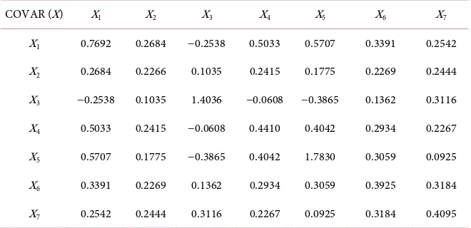
Table 3. Covariance matrix of government revenue.

COVAR (X) X1 X2 X3 X4 X5 X6 X7

X1 0.7692 0.2684 −0.2538 0.5033 0.5707 0.3391 0.2542

X2 0.2684 0.2266 0.1035 0.2415 0.1775 0.2269 0.2444

X3 −0.2538 0.1035 1.4036 −0.0608 −0.3865 0.1362 0.3116

X4 0.5033 0.2415 −0.0608 0.4410 0.4042 0.2934 0.2267

X5 0.5707 0.1775 −0.3865 0.4042 1.7830 0.3059 0.0925

X6 0.3391 0.2269 0.1362 0.2934 0.3059 0.3925 0.3184

X7 0.2542 0.2444 0.3116 0.2267 0.0925 0.3184 0.4095

4. Numerical Results

In this section, we implement the Markowitz model for Mongolian economy. We examine government budget revenue structure which depends on seven types of tax and nontax revenues.

Variable xi is the weight of i-th tax revenue in the portfolio. The Mongolian

government budget consists of the following revenues such as income tax, social security contributions, property taxes, taxes on domestic goods and services, taxes on foreign trade, other taxes and non-tax revenues. Table 4 shows the ini-tial values of variables as well as the optimal solution of problem (1)-(4) found by the conditional gradient method on MATLAB.

(7)

[image:7.595.212.541.89.223.2]

DOI: 10.4236/ib.2019.113004 48 iBusiness

Table 4. Solution.

Name Initial value Optimal value Change

Income tax 0.255 0.227 −2.8%

Social security contributions 0.118 0.115 −0.3% Property taxes 0.005 0.018 1.3% Taxes on domestic goods & services 0.296 0.194 −10.2%

Taxes on foreign trade 0.063 0.040 −2.3%

Other taxes 0.071 0.147 7.6%

Non-tax revenue 0.192 0.260 6.8%

5. Conclusion

We have tested the Markowitz model on Mongolian economic data in order to define optimal structure of the government revenue which consists of 7 com-ponents. Since the variance minimization problem was convex quadratic, for solving the problem we have applied the conditional gradient method coded in MATLAB. The numerical solution was obtained. In the same way, we can sider the problem of maximizing the government return subject to variance con-straint. But it will be discussed in the next paper.

Acknowledgements

This work was supported by the research grant P2018-3588 of National Univer-sity of Mongolia.

Conflicts of Interest

The authors declare no conflicts of interest regarding the publication of this pa-per.

References

[1] Markowitz, H. (1952) Portfolio Selection. The Journal of Finance, 7, 77-91.

https://doi.org/10.1111/j.1540-6261.1952.tb01525.x

[2] Fernholz, R.E. (2002) Stochastic Portfolio Theory, Volume 48. Springer Verlag, New York. https://doi.org/10.1007/978-1-4757-3699-1

[3] Homan, M., Brochu, E. and de Freitas, N. (2011) Portfolio Allocation for Bayesian Optimization. In:Heckerman, D. and Mamdani, A., Eds., Uncertainty in Artificial In-telligence, Elsevier, ‎Amsterdam, 327-336.

[4] Branke, J., Scheckenbach, B., Stein, M., Deb, K. and Schmeck, H. (2009) Portfolio Optimization with an Envelope-Based Multi-Objective Evolutionary Algorithm. Eu-ropean Journal of Operational Research, 199, 684-693.

https://doi.org/10.1016/j.ejor.2008.01.054

[5] Deniz, E. (2009) Multi-Period Scenario Generation to Support Portfolio Optimiza-tion. PhD Thesis, Rutgers, The State University of New Jersey, New Brunswick, NJ. [6] Daly, J., Crane, M. and Ruskin, H.J. (2008) Random Matrix Theory Filters in

(8)

Mechan-DOI: 10.4236/ib.2019.113004 49 iBusiness

ics and Its Applications, 387, 4248-4260.

https://doi.org/10.1016/j.physa.2008.02.045

[7] Christine Strauss (2001) Ant Colony Optimization in Multi Objective Portfolio Se-lection. 4th Metaheuristics International Conference,Porto, Portugal, 16-20 July 2001, 243-248.

[8] Geyer, A., Hanke, M. and Weissensteiner, A. (2009) A Stochastic Programming Ap-proach for Multi-Period Portfolio Optimization. Computational Management Science, 6, 187-208.https://doi.org/10.1007/s10287-008-0089-9

[9] Hester, D.D. and James, T. (1967) Risk Aversion and Portfolio Choice. John Wiley and Sons, Inc., New York.

[10] Nocedal, J. and Wright, S.J. (1999) Numerical Optimization. Springer Series in Op-erations Research. 2nd Edition, Springer, Berlin. https://doi.org/10.1007/b98874

[11] Chen, W., Zhang, R.-T., Cai, Y.-M. and Xu, F.-S. (2006) Particle Swarm Optimiza-tion for Constrained Portfolio SelecOptimiza-tion Problems. 2006 International Conference on Machine Learning and Cybernetics, Dalian,13-16 August 2006, 2425-2429.

https://doi.org/10.1109/ICMLC.2006.258773

[12] Black, F. and Litterman, R. (1992) Global Portfolio Optimization. Financial Analysts Journal, 48, 28-43.https://doi.org/10.2469/faj.v48.n5.28

[13] Bolshakova, I., Girlich, E. and Kovalev, M. (2009) Portfolio Optimization Problems: A Survey. Otto-von-Guericke University Magdeburg, Germany.

[14] Sharpe, W.F. (1964) Capital Asset Prices: A Theory of Market Equilibrium under Conditions of Risk. The Journal of Finance, 19, 425-442.

https://doi.org/10.1111/j.1540-6261.1964.tb02865.x

[15] Christodoulakis, G.A. (2002) Bayesian Optimal Portfolio Selection: The Black-Litterman Approach. Notes for Quantitative Asset Pricing, MSc. Mathematical Trading and Finance, City, University of London, London.

[16] Walters, J. (2009) The Black-Litterman Model in Detail. Harvard Management Com-pany,Boston, MA, 16-67.

[17] Zhou, G. (2009) Beyond Black-Litterman: Letting the Data Speak. The Journal of Portfo-lio Management, 36, 36-45.https://doi.org/10.3905/JPM.2009.36.1.036

[18] Boyd, S. and Vandenberghe, L. (2009) Convex Optimization. 7th Edition, Cam-bridge University Press, CamCam-bridge.

[19] Parpas, P., Rustem, B., Wieland, V. and Zakovie, S. (2006) Mean Variance Optimi-zation of Non-Linear Systems and Worst-Case Analysis. Computational Optimiza-tion and ApplicaOptimiza-tions, 43, 235-259. https://doi.org/10.1007/s10589-007-9136-7

[20] Guastaroba, G., Mitra, G. and Speranza, M.G. (2011) Investigating the Effectiveness of Robust Portfolio Optimization Techniques. Journal of Asset Management, 12, 260-280.

https://doi.org/10.1057/jam.2011.7

[21] Greyserman, A., Jones, D. and Strawderman, W. (2006) Portfolio Selection Using Hierarchical Bayesian Analysis and MCMC Methods. Journal of Banking & Finance, 30, 669-678. https://doi.org/10.1016/j.jbankfin.2005.04.008

[22] Roudier, F. (2006) Portfolio Optimization and Genetic Algorithms. Master’s Thesis, Swiss Federal Institute of Technology (ETM), Zurich.

(9)

DOI: 10.4236/ib.2019.113004 50 iBusiness [24] Lin, D. and Li, X. (2005) A Genetic Algorithm for Solving Portfolio Optimization

Problems with Transaction Costs and Minimum Transaction Lots. In: Wang, L., Chen, K. and Ong, Y., Eds., Advances in Natural Computation, Springer, Berlin, Hei-delberg, 808-811. https://doi.org/10.1007/11539902_99

[25] Thong, V. (2007) Constrained Markowitz Portfolio Selection Using Ant Colony Optimization. Erasmus University, Rotterdam.

[26] Mishra, S.K., Panda, G. and Meher, S. (2009) Multi-Objective Particle Swarm Opti-mization Approach to Portfolio OptiOpti-mization. 2009 World Congress on Nature and Biologically Inspired Computing, Coimbatore, India, 9-11 December 2009, 1612-1615.

https://doi.org/10.1109/NABIC.2009.5393659