Refinement and Quantification of Terrain Induced Effects on Global Gravity Data

ISSN Online: 2156-8367 ISSN Print: 2156-8359

DOI: 10.4236/ijg.2019.105030 May 8, 2019 513 International Journal of Geosciences

Refinement and Quantification of

Terrain-Induced Effects on Global Gravity Data

Ojima I. Apeh

, Elochukwu C. Moka, Victus N. Uzodinma, Elijah S. Ebinne

Department of Geoinformatics & Surveying, University of Nigeria, Enugu Campu, Enugu, Nigeria

Abstract

The geodetic and geophysical applications of Earth Gravity Field parameters computed from Global Geopotential Models (GGMs) are quite on the in-crease despite the inherent commission and omission errors of these models. In view of this, this study focuses on refining and quantifying terrain-induced effects on Bouguer gravity anomalies computed directly from a total of seven recent GGMs. In the study, the Residual Terrain Model (RTM) tech-nique was used to estimate the residual terrain effects that were added to the GGM-computed Bouguer gravity anomalies at the sixty test points in Enugu State, Nigeria. The computed residual terrain effects range from −24.6 to 37.5 mgal while the percentage of the omission errors of the GGMs based on their Root-Mean-Square (RMS) differences ranges from 7.8% to 44.7%. It can be concluded that GGM-refined Bouguer gravity anomalies are better in accu-racy than the unrefined GGM-computed Bouguer gravity anomalies and hence there is need for accurate height information in the development of GGMs. We, therefore, recommend that refined Bouguer gravity anomalies obtained from HUST-Grace2016s, EIGEN-6C4 and GECO that gave best im-provement amongst the seven GGMs under consideration should be used to supplement the available terrestrial Bouguer anomalies for geodetic and geo-physical applications within the study area.

Keywords

Bouguer Gravity Anomalies, Global Geopotential Models, Refined Bouguer Anomalies, Residual Terrain Model (RTM) Effects

1. Introduction

A GGM is a mathematical approximation to the external gravitational potential of an attracting body. It consists of a set of numerical values for certain

parame-How to cite this paper: Apeh, O.I., Moka, E.C., Uzodinma, V.N. and Ebinne, E.S. (2019) Refinement and Quantification of Terrain-Induced Effects on Global Gravity Data. International Journal of Geosciences, 10, 513-526.

https://doi.org/10.4236/ijg.2019.105030 Received: March 27, 2019

Accepted: May 5, 2019 Published: May 8, 2019

Copyright © 2019 by author(s) and Scientific Research Publishing Inc. This work is licensed under the Creative Commons Attribution International License (CC BY 4.0).

http://creativecommons.org/licenses/by/4.0/

DOI: 10.4236/ijg.2019.105030 514 International Journal of Geosciences ters or functionals, the statistics of the errors associated with these values and a collection of mathematical expressions and algorithms [1]. Nowadays, GGMs are serving as good alternatives for modeling the gravity field of the earth espe-cially in regions devoid of, or having inadequate terrestrial gravity data coverage. But they are subject to omission and commission errors. The commission error is produced by the statistical errors of the fully normalized spherical harmonic coefficients while the omission error in spherical harmonic expansion comprises high-frequency gravity field signals that cannot be represented by a truncated spherical harmonic series expansion, that is, all gravity field features occurring at scales finer than the GGM’s spatial resolution [2] [3]. The contribution of long-wavelengths of the gravity field signals to the gravity anomaly is computed from GGM while the short-wavelengths are computed from Digital Elevation Model (DEM) since the Earth’s topography is the main source of high-frequency gravity field [4]. Where the DEM is not very accurate in relation to the ac-tual/observed terrain values, the effect is reflected in the accuracy of the com-puted parameter of earth gravity field being sought.

It, then, becomes necessary to enhance/improve the accuracy of GGM-computed gravity data for effective geodetic and geophysical applications in any area. In-ternational Centre for Gravity Earth Models (ICGEM) [5] publishes, from time to time, GGMs that have been developed by geoscientists. It is true that many functionals of the gravity field (e.g. geoid undulation, height anomaly, gravity anomaly, Absolute gravity, etc.) can be computed from the ICGEM website us-ing any GGM of interest but these computed quantities need to be evaluated and refined using terrestrial data in order to improve their accuracy for geosciences applications in any locality. This is necessary because the accuracy and the re-solving power of the data used in the development of a GGM determine its ac-curacy and resolution.

Many authors [6] [7] [8] [9] [10] have evaluated some of the GGMs using ter-restrial data of their locality and discovered relatively high standard deviations or Root-Mean-Square (RMS) differences in gravity anomaly between the two of around 10 mgal and even more. The reason for this large difference has often been attributed to the so-called omission and commission errors inherent in the GGMs; possible systematic errors in the observed terrestrial data and topo-graphic bias. There is need to quantify the size of these omission errors. In fact, any of the Digital Elevation Models (DEMs) used to provide height information in gravity reduction may not adequately represent the local topography of an area because of the interpolation and extrapolation errors inherent in DEMs

DOI: 10.4236/ijg.2019.105030 515 International Journal of Geosciences

[15] [16].

There is sparse distribution of gravity data within the study area and there is need for both denser distribution of gravity data as well as more accurate know-ledge of gravity field in the study area for several geosciences and environmental applications. Although embarking on more terrestrial gravity observation is time-consuming, very expensive and laborious yet that may not (considering a large study area) produce sufficiently dense network of gravity data distribution required in several geosciences and environmental applications like oil, gas and mineral exploration, geoid modelling, deformation studies, geophysical survey-ing, engineering projects and many others. Hence, this study focuses on refining Bouguer gravity anomalies computed from some of the recent GGMs in order to improve their accuracy and to estimate the GGMs signal omission errors from the RMS differences between the directly computed Bouguer gravity anomalies and that of the refined Bouguer gravity anomalies obtained after applying resi-dual terrain effects. As a result of the paucity of terrestrial gravity data in the study area and the relatively high Root-Mean-Square (RMS) differences between the GGM-computed Bouguer gravity anomalies and that of the terrestrially ob-served Bouguer gravity anomalies as shown in [6], we refined the GGM-computed Bouguer gravity anomalies to see if they can be used either alone or in combina-tion with available terrestrial Bouguer gravity data for some engineering, geo-detic and geophysical applications within the study area.

2. Materials and Method

2.1. Study Area

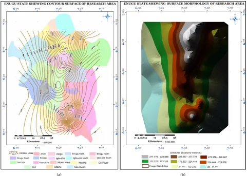
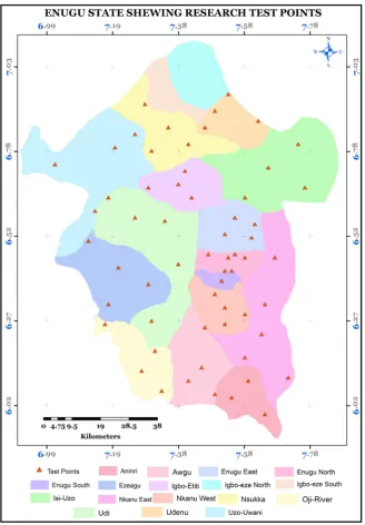
The study area (Figure 1) is situated within longitudes 6˚49'E - 7˚51'E and lati-tudes 6˚01'N - 7˚12'N respectively. It has an average range of elevation of 57.40 m to 598.87 m reflecting topographic lows and highs. A good part of the area contains coal deposit. The sixty (60) test points selected for this study are distri-buted within the study area as shown in Figure 2

2.2. Data

The data used in this study were obtained from various sources as listed in Table 1. There are seven (7) GGMs used in this study, and these were selected based on the sources of data used in their development. These GGMs were also previously evaluated at the study area [6]. They consist of four (4) Satellite-based GGMs and three (3) combined Satellite, Gravity data and Altimetry data GGMs. The different GGMs are characterized based on the input data, method of calcula-tion, the degree and order of expansion which determine the resolution as well as the other things modeled as given in Table 2.

Nigeria Geological Survey Agency (NGSA) provided the terrestrial Bouguer gravity data used in this study and as published

DOI: 10.4236/ijg.2019.105030 516 International Journal of Geosciences

(a) (b)

Figure 1. Study area (Source: Enugu Ministry of Lands and Surveys).

Table 1. Data sources.

S/N0 Data Sources

1 Terrestrial Bouguer gravity Nigerian Geological Survey Agency (NGSA) 2 Computed Bouguer gravity ICGEM website

3 Terrestrial DEM Enugu State ministry of lands and surveys 4 Reference DEM ICGEM website

5 Global Gravity Field Models (GGMs) ICGEM website

Table 2. Characteristics of the seven GGMs used in this study.

Model (d/o) Source of Data Reference HUST-Grace2016s (160) S(Grace) [17]

ITU_GGC16 (280) S(Grace, Goce) [18]

EIGEN-6C4 (2190) S(Goce, Grace, Lageous), G, A [19]

GGM05G (240) S(Grace, Goce) [20]

GECO (2190) S(Goce), EGM2008 [21]

EGM2008 (2190) S(GRACE), G, A [22]

GO_CONS_GCF_2_SPW_R4 (280) S(Goce) [23]

DOI: 10.4236/ijg.2019.105030 517 International Journal of Geosciences Figure 2. Location of the test points.

1) Lacoste and Romberg (G-512) gravimeter (±0.01 mgal);

2) FA-181 Wallace, Tiernan and Brunton Barometric altimeters (±1 m); 3) American Paulin System MDM-5 (±0.5 m);

4) Sling Psychrometer;

5) Garmin Csx 76 GPS (±3 m).

psyc-DOI: 10.4236/ijg.2019.105030 518 International Journal of Geosciences hrometer was used to measure the Air temperature while the relative humidity used in correcting the barometric readings was determined from the psychro-metric chart. The result of this survey shows a good correlation between the Bouguer anomalies and the surface geology of Enugu State when compared with the existing geological map

(http://www.ngsa-nig.org/content/regional-gravity-survey-enugu-state).

2.3. Method

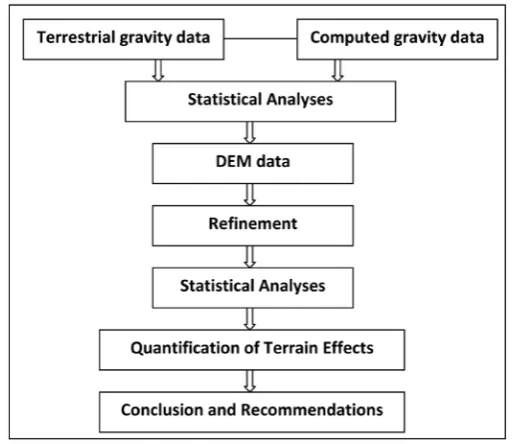
The method used in carrying out this study is designed as shown in Figure 3

Bouguer gravity anomalies obtained for each of the seven GGMs were com-puted on-line from the calculation service of the International Centre for Gravity Earth Models (http://icgem.gfz-potsdam.de/tom_longtime). All the computa-tions were carried out on Geodetic Reference System 1980 ellipsoid and in the

Mean Tide system while the box for the zero degree term remained unchecked.

The GGMs were truncated at their maximum degree of expansion (low-pass fil-tering) and there was no Gaussian filtering of any sort. Among others, it requires geodetic coordinates of each of the test points to be inputted [5]. For these GGMs, the Bouguer gravity anomalies are calculated by the spherical approxi-mation (Equation (1)) of the classical gravity anomalies minus 2πGρH [27].

(

)

(

)

(

)

(

)

2 0 0

, , 1 sin cos sin

l

l l T T

sa l m lm lm lm

GM R

g r l P C m S m

r r

λ ϕ ₌   ₌ ϕ λ λ

∆ = _{ } − +

 

∑

∑

where; ∆gsa = Gravity anomaly in spherical approximation, GM = geocentric

gravitational constant, T W U

lm lm lm

C =C −C , SlmT =SlmW −SlmU ; T lm

C , SlmT =

coeffi-cients of the disturbing potential. l = degree, m = order, r = radius (geocentric distance), λ _{= spherical longitude,} ϕ _{= polar distance (spherical co-latitude),}

max

l = maximum degree of expansion.

DOI: 10.4236/ijg.2019.105030 519 International Journal of Geosciences The ETOPO1 topography model (Equation (2)) is the spherical harmonic ex-pansion of the (1’ × 1’) grid of ETOPO1 (version: Ice Surface) of Earth’s topo-graphy used in the computation of orthometric heights in ICGEM website [27]. The reference elevation surfaces were computed in correspondence to the de-gree/order of each of the GGMs using the calculation service of the International Centre for Global Earth Models [5].

(

)

(

)

(

)

0 0

, ll lm lm sin lm cos lm sin

H λ ϕ =R

∑ ∑

where; H

(

)

topo

lm

S =

Coefficients of expansion.

Residual Terrain Model (RTM) effects refer to the effects of the topographic irregularities with respect to a mean or reference surface. The two digital eleva-tion models, a DTM file (Terrestrial DEM) and a reference DTM file (Reference DEM), were used in the outer and inner zones respectively for the computation of RTM effects. The Terrestrial DEM was the cloud of LIDAR (Light Detection And Ranging) points acquired over the study area by the Enugu State government.

GRAVSOFT programs (TCFOUR, TCGRID and SELECT) were used for the computation of the RTM effects [28]. SELECT was used to prepare 10 arc-seconds of average height grid for the two DTM files which cover latitudes 5.96˚N - 6.92˚N and longitudes 7.08˚E - 7.80˚E. TCGRID was used to average the refer-ence DEM into a referrefer-ence height grid and in order to obtain optimal smooth-ing: a reference height grid resolution of 100 km was used. TCFOUR (Computa-tion of terrain effects by Fast Fourier Technique (FFT) convolu(Computa-tions in planar approximation) was used to compute Residual Terrain Model (RTM) effects in mode 4 (which computes the effects of the topographic irregularities with refer-ence to a mean surface). The coordinates of the South-West corner grid was 5.96˚ (latitude), 6.92˚ (longitude). The distance of computation ranges from 0 to 999.9 km. The details on how to carry out the computation of RTM effects using GRAVSOFT programs are contained in “An Overview Manual for the GRAVSOFT Geodetic Gravity Field Modeling Programs” by [28].

The absolute values of the RTM effects at each of the test points were added to the Bouguer anomalies computed from each of the seven GGMs to obtain the refined Bouguer anomalies at each of the sixty (60) test points. The descriptive statistics of the computed and refined Bouguer gravity anomalies were deter-mined. The percentage of the signal omission errors of each of the seven GGMs were estimated from the RMS differences using Equation (3).

Refined Computed

Computed

RMS RMS

Percentage of omission error 100

RMS

−

= × ₍₃₎

where; RMSRefined = Root-Mean-Square obtained from the difference in Refined

and terrestrial Bouguer anomalies, RMSComputed = Root-Mean-Square obtained

from the difference in computed and terrestrial Bouguer anomalies.

3. Results and Discussions

DOI: 10.4236/ijg.2019.105030 520 International Journal of Geosciences presented in Table 3. Comparing the GGM-computed Bouguer gravity anoma-lies (without the RTM effects) with the directly measured gravity, the RMS dif-ference ranges from 9.6 to 17.9 mgal.

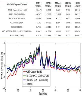
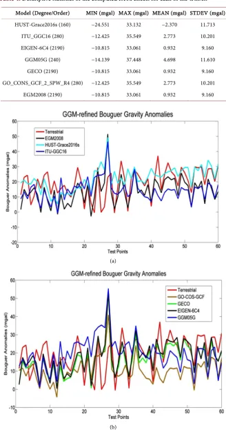
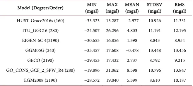
The graph in Figure 4 shows the results of the computed RTM effects at each of the sixty test points while Table 4 shows the descriptive statistics.

It is observed that the values of RTM effects are the same for EIGEN 6C4/EGM2008/GECO and ITU_GGC/GO_CONS_GCF_2_SPW_R4. This is be-cause they have the same maximum degree of expansion thereby having the same reference or mean elevation as computed from ETOPO1 topography mod-el.

The absolute values of the residual terrain effects at each of the test points were added to the Bouguer anomalies computed from each of the seven GGMs to obtain the refined Bouguer anomalies at each of the test points. The refined Bouguer anomalies, as obtained in this study, are shown in Figure 5 while Table 5 shows the descriptive statistics.

Table 3. Statistical results of GGM-computed and the terrestrial Bouguer anomalies.

Model (Degree/Order) _(mgal) MIN _(mgal) MAX MEAN _(mgal) STDEV _{(mgal) (mgal)} RMS HUST-Grace2016s (160) −10.175 23.572 6.687 7.970 10.440 ITU_GGC16 (280) −4.343 27.035 12.805 6.628 14.515 EIGEN-6C4 (2190) −1.189 19.165 8.133 5.013 9.613

GGM05G (240) −6.313 22.950 8.596 6.866 11.058 GECO (2190) 0.708 20.826 9.471 4.520 10.567 GO_CONS_GCF_2_SPW_R4 (280) 0.451 31.801 16.600 6.329 17.896 EGM2008 (2190) 0.815 22.434 12.134 4.371 12.993

DOI: 10.4236/ijg.2019.105030 521 International Journal of Geosciences Table 4. Descriptive statistics of the computed RTM effects for each of the GGMs.

Model (Degree/Order) MIN (mgal) MAX (mgal) MEAN (mgal) STDEV (mgal) HUST-Grace2016s (160) −24.551 33.132 −2.370 11.713

ITU_GGC16 (280) −12.425 35.549 2.773 10.201 EIGEN-6C4 (2190) −10.815 33.061 0.932 9.160

GGM05G (240) −14.139 37.448 4.698 11.610 GECO (2190) −10.815 33.061 0.932 9.160 GO_CONS_GCF_2_SPW_R4 (280) −12.425 35.549 2.773 10.201

EGM2008 (2190) −10.815 33.061 0.932 9.160

(a)

(b)

DOI: 10.4236/ijg.2019.105030 522 International Journal of Geosciences Table 5. Statistical results of the differences between the refined and terrestrial Bouguer anomalies at the sixty (60) test points.

Model (Degree/Order) _(mgal) MIN _(mgal) MAX MEAN _(mgal) STDEV _{(mgal) (mgal)} RMS HUST-Grace2016s (160) −33.323 13.287 −2.977 10.926 11.331 ITU_GGC16 (280) −24.507 26.296 4.803 11.191 12.195 EIGEN-6C 4(2190) −30.655 16.856 1.398 8.843 8.954

GGM05G (240) −35.457 17.608 −0.478 13.448 13.456 GECO (2190) −29.453 17.432 2.737 8.792 9.215 GO_CONS_GCF_2_SPW_R4 (280) −19.896 31.062 8.598 10.796 13.847

EGM2008 (2190) −28.572 19.040 5.399 8.610 10.187

Adding the signal omission error estimates from RTM to each of the GGMs significantly reduced the RMS differences between the computed and the terre-strial Bouguer gravity anomalies at the sixty (60) test points. Comparing Table 5

with Table 2, it is pertinent to note, and as corroborated in other studies, that refined Bouguer anomalies have better statistical results than the computed Bouguer anomalies [3] [10] [11] [12] [13]. This is so because there is always a bias between DEM data and terrestrial data as a result of the great deviations in gradient of the undulating terrain when point values are compared to mean val-ues such as reference DEM used in the GGMs.

Equation (3) was applied in the computation of percentage of omission error of the GGM-derived Bouguer gravity anomalies computed from each of the GGMs and the statistical results are shown in Table 6.

Considering the sixty (60) test points, the RTM effects improved the modeling of ITU_GGC16, EIGEN-6C4, GECO, GO_CONS_GCF_2_SPW_R4, EGM2008 by 16.54%, 7.82%, 15.25%, 23.06% and 21.60% respectively while it decreased the modeling of HUST-Grace2016s, GGM05G by 8.30% and 21.32% respectively on the average. Interestingly, after a careful examination of the results presented in

Figure 5, we observed that if the points (PtID: 20, 23, 25, 26, 27, 29, 33, 40) that are 399 m and above in elevation are removed, the statistical results would then become better as shown in Table 7 and the percentage of omission errors will change considerably for all the GGMs as shown in Table 8. This confirms the fact that the values of RTM effects are large on the mountains and these values deteriorated the statistical results of sixty (60) test points on the average. It is no-ticed that the RMS differences and the percentage of the omission errors reduced considerably as shown in Table 7 and Table 8.

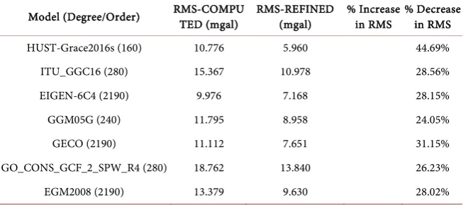
Considering the fifty-two (52) test points, the RTM effects improved the mod-eling of HUST-Grace2016s, ITU_GGC16, EIGEN-6C4, GGM05G, GECO, GO_CONS_GCF_2_SPW_R4, EGM2008 by 44.19%, 28.15%, 24.05%, 31.15%, 30.49%, 26.23% and 28.02% respectively on the average.

DOI: 10.4236/ijg.2019.105030 523 International Journal of Geosciences Table 6. Percentage of refinement for the RMS difference of the computed and refined Bouguer anomalies at the sixty (60) points.

Model (Degree/Order) RMS-COMPUTED RMS-REFINED % Increase in RMS % Decrease in RMS HUST-Grace2016s (160) 10.44 11.307 8.30%

ITU_GGC16 (280) 14.515 12.114 16.54% EIGEN-6C4 (2190) 9.613 8.861 7.82%

GGM05G (240) 11.058 13.416 21.32%

GECO (2190) 10.567 8.961 15.20% GO_CONS_GCF_2_SPW_R4 (280) 17.896 13.77 23.06% EGM2008 (2190) 12.993 10.187 21.60%

Table 7. Statistical results of the difference between refined and terrestrial Bouguer ano-malies at the fifty-two (52) points.

Model (Degree/Order) _(mgal) MIN _(mgal) MAX MEAN _(mgal) STDEV _{(mgal) (mgal)} RMS HUST-Grace2016s (160) −13.774 13.287 0.644 5.978 5.960

ITU_GGC16 (280) −11.662 26.296 8.086 7.339 10.978 EIGEN-6C4 (2190) −10.562 16.856 3.754 6.083 7.168

GGM05G (240) −13.195 17.608 3.801 8.094 8.958 GECO (2190) −7.822 17.432 5.330 5.437 7.651 GO_CONS_GCF_2_SPW_R4 (280) −6.868 31.062 11.751 7.125 13.840

EGM2008 (2190) −8.558 19.040 7.766 5.589 9.630

Table 8. Percentage of refinement for the RMS difference of the computed and refined Bouguer anomalies at the fifty-two (52) points.

Model (Degree/Order) RMS-COMPU_{TED (mgal)} RMS-REFINED _(mgal) % Increase _{in RMS} % Decrease _{in RMS} HUST-Grace2016s (160) 10.776 5.960 44.69%

ITU_GGC16 (280) 15.367 10.978 28.56% EIGEN-6C4 (2190) 9.976 7.168 28.15% GGM05G (240) 11.795 8.958 24.05% GECO (2190) 11.112 7.651 31.15% GO_CONS_GCF_2_SPW_R4 (280) 18.762 13.840 26.23% EGM2008 (2190) 13.379 9.630 28.02%

prob-DOI: 10.4236/ijg.2019.105030 524 International Journal of Geosciences lem. The importance of accurate height information in the development of GGMs is clearly illustrated in this study since it can greatly influence the accu-racy of the computed earth gravity parameters such as Bouguer gravity anoma-lies.

4. Conclusion and Recommendations

This study, which aimed at refining and quantifying terrain-induced effects on global gravity data, applied GRAVSOFT Fast Fourier Technique (FFT) to com-pute Residual Terrain Model (RTM) effects which were used in refining the sig-nal omission errors inherent in the GGMs. The RTM technique is capable of modeling major parts of high-resolution GGM signal omission errors inherent in the GGMs and can improve geodetic and geophysical applications of the computed earth field parameters. Bouguer gravity anomalies are very useful source for interpretation and analysis of subsurface density anomalies and they can be used in accurate determination of the geoid in geodesy when refined.

The relatively high values of the Root-Mean-Square differences of the refined Bouguer gravity anomalies are resulting from the commission errors inherent in the GGMs; possible systematic errors in the observed terrestrial Bouguer gravity anomalies and possible deviations of the Terrestrial DEM from the geoid. This is still open to further studies.

Based on the results obtained from this study, we conclude that:

1) Signal omission errors (terrain-induced effects) can greatly deteriorate the accuracy of parameters computed from GGMs;

2) GGM-refined Bouguer gravity anomalies are better in accuracy than the GGM-computed Bouguer gravity anomalies;

3) EIGEN-6C4 and GECO GGM-refined Bouguer anomalies could be used to supplement the terrestrial Bouguer anomalies in some Local Government Areas of Enugu State for geodetic and geophysical applications;

4) HUST-Grace2016s GGM-refined Bouguer anomalies could be used to sup-plement the terrestrial Bouguer anomalies in locations whose elevations are less than 399 m above mean sea level;

5) Accurate earth’s gravity field, high precision and high resolution geoid may not be achievable from these seven GGMs at least for the study area;

6) Remodelling/tailoring of these GGMs using local terrestrial gravity data is required to enhance their accuracy in Enugu State, Nigeria.

Acknowledgements

The authors are very grateful to the Nigerian Geological Survey Agency (NGSA) for providing terrestrial gravity data for this study.

Conflicts of Interest

DOI: 10.4236/ijg.2019.105030 525 International Journal of Geosciences

References

[1] Pavlis, N.K. (2006) Global Gravitational Modeling: An Overview Considering Cur-rent and Future Dedicated Gravity Mapping Missions. IGes Geoid School 2006, the Determination and Use of the Geoid, Copenhangen, 19-23 June 2006.

[2] Torge, W. (2001) Geodesy. 3rd Edition, de Gruyter, Berlin, New York. https://doi.org/10.1515/9783110879957

[3] Hirt, C., Marti, U., Bürki, B. and Featherstone, W.E. (2010) Assessment of EGM2008 in Europe Using Accurate Astrogeodetic Vertical Deflections and Omis-sion Error Estimates from SRTM/DTM2006.0 Residual Terrain Model Data. Journal of Geophysical Research, 115, B10404.https://doi.org/10.1029/2009JB007057 [4] Forsberg, R. (1984) A Study of Terrain Reductions, Density Anomalies and

Geo-physical Inversion Methods in Gravity Field Modeling. Dept. of Geodetic Science and Surveying, the Ohio State University, Colombus, Report No. 355.

https://doi.org/10.21236/ADA150788

[5] Barthelmes, F. and Köhler, W. (2016) International Centre for Global Earth Models (ICGEM). Journal of Geodesy, 90, 907-1205.

https://doi.org/10.1007/s00190-016-0948-z

[6] Apeh, O.I., Moka, E.C. and Uzodinma, V.N. (2018) Evaluation of Gravity Data De-rived from Global Gravity Field Models Using Terrestrial Gravity Data in Enugu State, Nigeria. Journal of Geodetic Science, 8, 145-153.

https://doi.org/10.1515/jogs-2018-0015

[7] Ibrahim Yahaya, S. and El Azzab, D. (2018) High-Resolution Residual Terrain Model and Terrain Corrections for Gravity Field Modelling and Geoid Computa-tion in Niger Republic. Geodesy and Cartography, 44, 89-99.

https://doi.org/10.3846/gac.2018.3787

[8] Odera, P.A. (2016) Assessment of EGM2008 Using GPS/Leveling and Free-Air Gravity Anomalies over Nairobi County and Its Environs. South African Journal of Geomatics, 5, 17-30. https://doi.org/10.4314/sajg.v5i1.2

[9] Saari, T. and Bilker-Koivula, M. (2015) Evaluation of GOCE-Based Global Geoid Models in Finnish Territory. EGU General Assembly 2015, Vienna, 12-17 April 2015, Article ID: 4165.

[10] Šprlák, M., Gerlach, C., Omang, O. and Pettersen, B. (2011) Comparison of GOCE Derived Satellite Global Gravity Models with EGM2008, the OCTAS Geoid and Terrestrial Gravity Data: Case Study for Norway. Proceedings of the 4th Interna-tional GOCE User Workshop, Munich, 31 March-1 April 2011.

[11] Merry, C.L. (2003) DEM-Induced Errors in Developing a Quasi-Geoid Model for Africa. Journal of Geodesy, 77, 537-542.https://doi.org/10.1007/s00190-003-0353-2 [12] Tong, L.T. and Guo, T.R. (2007) Gravity Terrain Effect of the Seafloor Topography

in Taiwan. Terrestrial Atmospheric and Oceanic Sciences, 18, 699. https://doi.org/10.3319/TAO.2007.18.4.699(T)

[13] Wang, J.-H. and Geng, Y. (2015) Terrain Correction in the Gradient Calculation of Spontaneous Potential Data. Chinese Journal of Geophysics, 58, 654-664.

https://doi.org/10.1002/cjg2.20202

[14] Sampietro, D., Sona, G. and Venuti, G. (2007) Residual Terrain Correction on the Sphere by an FFT Algorithm. 1st International Symposium of the International Gravity Field Service, Istanbul, 28 August-1 September 2006.

DOI: 10.4236/ijg.2019.105030 526 International Journal of Geosciences [16] Leaman, D.E. (1998) The Gravity Terrain Correction-Practical Considerations.

Ex-ploration Geophysics, 29, 467-471.https://doi.org/10.1071/EG998467

[17] Zhou, H., Luo, Z., Zhou, Z., Zhong, B. and Hsu, H. (2016) A New GRACE-Only Static Gravity Field Model: HUST-Grace2016s.

[18] Akyilmaz, O., Ustun, A., Aydin, C., Arslan, N., Doganalp, S., Guney, C., Mercan, H., Uygur, S.O., Uz, M. and Yagci, O. (2016a) ITU_GGC16 the Combined Global Gravity Field Model Including GRACE & GOCE Data up to Degree and Order 280. [19] Förste, C., Bruinsma, S.L., Abrikosov, O., Lemoine, J.-M., Marty, J.C., Flechtner, F.,

Balmino, G., Barthelmes, F. and Biancale, R. (2015) EIGEN-6C4 the Latest Com-bined Global Gravity Field Model Including GOCE Data up to Degree and Order 2190 of GFZ Potsdam and GRGS Toulouse.

[20] Bettadpur, S., Ries, J., Eanes, R., Nagel, P., Pie, N., Poole, S., Richter, T. and Save, H. (2015) Evaluation of the GGM05 Mean Earth Gravity Models. EGU General As-sembly 2015, Vol. 17, Vienna, 12-17 April 2015, EGU2015-4153.

[21] Gilardoni, M., Reguzzoni, M. and Sampietro, D.(2015) GECO: A Global Gravity Model by Locally Combining GOCE Data and EGM2008. Studia Geophysica et Geodaetica, 60, 228-247.https://doi.org/10.1029/2003GL018025

[22] Pavlis, N.K., Holmes, S.A., Kenyon, S.C. and Factor, J.K. (2008) An Earth Gravita-tional Model to Degree 2160: EGM2008. 2008 General Assembly of the European Geoscience Union, Vienna, 13-18 April 2008, 1-37.

https://doi.org/10.1190/1.3063757

[23] Gatti, A., Reguzzoni, M., Migliaccio, F. and Sanso, F. (2014) Space-Wise Grids of Gravity Gradients from GOCE Data at Nominal Satellite Altitude. GOCE User Workshop, Paris, 25-28 November 2014.

[24] Morelli, C., Gantar, C., McConnell, R.K., Szabo, B. and Uotila, U. (1972) The International Gravity Standardization Net 1971 (IGSN 71). Osservatorio Geofisico Sperimentale Trieste (Italy).

[25] Osazuwa, I.B. (1985) The Establishment of a Primary Gravity Network for Nigeria. PhD Thesis, Ahmadu Bello University, Zaria.

[26] Osazuwa, I.B. (1992a) The Nigerian Standard Calibration Line. Survey Review, 31, 397-408.https://doi.org/10.1179/sre.1992.31.245.397

[27] Barthelmes, F. (2013) Definition of Functionals of the Geopotential and Their culation from Spherical Harmonic Models: Theory and Formulas Used by the Cal-culation Service of the International Centre for Global Earth Models (ICGEM). Scientific Technical Report STR09/02, Revised Edition.