Comprehensive Research on the Origin of the Solar System
Structure by Quantum-Like Model
Qingxiang Nie
College of Physics and Electronics, Shandong Normal University, Jinan, China E-mail: [email protected]
Received April 10, 2011; revised May 17, 2011; accepted May 27, 2011
Abstract
A quantum-like model of gravitational system is introduced to explore the formation of the solar system structure. In this model, the chaos behavior of a large number of original nebular particles in a gravitational field can be described in terms of the wave function satisfying formal Schrödinger equation, in which the Planck constant is replaced by a constant g on cosmic scale. Numerical calculation shows that the ra-dial distribution density of the particles has the character of wave curves with decreasing amplitudes and elongating wavelengths. By means of this model, many questions of the solar system, such as the planetary distance, mass, energy, angular momentum, the distribution of satellites, the structure of the planetary rings, and the asteroid belt and the Kuiper belt etc., can be explained in reason. In addition, the abnormal rotations of Venus and Mercury can be naturally explained by means of the quantum-like model.
Keywords: Schrödinger Equation, Planetary Distances and Masses, Satellites Distribution, Rings Structure, Kuiper Belt, Asteroid Belt
1. Introduction
There are many quantization phenomena on cosmic scale in the solar system, such as the planetary distance, orbital energy and angular momentum, the distribution of regu-lar satellites of giant planets, planetary ring system, and so on. Among these phenomena, the planetary distance law, called Titius-Bode law [1], is the most famous one. Although this law has been studied for over two hundred years, its physical explanation remains open so far. Ti-tius-Bode law is generally denoted as
0.4 0.3 2n n
a , (1) where an is the planetary orbital semi-major axis in astronomical units (AU), n , 0, 1, 2, 4, 5 for the Mercury, Venus, Earth, Mars, Jupiter and Saturn. But Neptune and Pluto are not consistent with the law. Ti-tius-Bode law means the planetary distance into a quan-tization series. The series are later also denoted by for-mulas [2-11]
0 n
n
a a d or an1/and , (2) where a0 and d are constants and are given different values in different articles in order to fit in with the obser-vations. Although the two formulas are still imprecise, the
quantization series of the planetary orbits is more obvious. So some hypotheses on quantum theory of gravitational field have been continually raised [11-21]. The common view of these hypotheses is that the quantum mechanics theory can be applied not only to the microscopic field, but also possibly to the gravitational field in the cosmic scale, with the large scale Planck constants. Among these re-searchers, some used the analogy between the planetary orbits and Bohr-Sommerfeld quantization orbits, while others applied the Schrödinger equation or Schrödinger-like equation to planetary system. Despite some exciting results, the phenomena are far from being completely ex-plained due to the complexity of the formation and evolu-tion of the solar system. In addievolu-tion, some other phenom-ena, such as the planetary mass, energy, angular momen-tum, and the structure of rings, are rarely studied yet, and to explain them requires a uniform theory.
large to be dominated by quantum law.
By means of the Schrödinger-like equation of micro-scopic particles in the gravitational field, Nie et al. have made preliminary interpretations on the planetary dis-tance [17], the population of Kuiper belt objects [22], and the unusual rotation of Venus and Mercury [23]. This paper attempts to systematically illustrate the origin of the solar system structure including planetary distance and mass, distribution of regular satellites, the asteroid belt and Kuiper belt, the structure of rings and so on.
2. A Quantum Clue on the Solar System
The similarities between quantum mechanics and stochas-tic motion of parstochas-ticles have been nostochas-ticed in some early papers. Comisar (1965) has introduced a Brownian motion model to explain the behavior of electron described in quantum mechanics [24]. Nelson (1966) has given a deri-vationof the Schrödinger equation for an electron motion from the theory of Brownian motion [25]. Following Nel-son, Nottale et al. (1997) have applied a Schrödinger-like equation to planets in the solar system [21].
The quantization character of planetary orbits has been expressed in teams of Bohr orbit 2
0
n
a n a by some researchers (e.g., Yang [19], Agnese & Festa [20]), where a0 is the “Bohr radius” of planetary system with different values in various literatures, and n is the prin-cipal quantum number. The difficulty in applying Bohr orbit is that the values of n must be discrete integer in order to fit the planets and satellites.
If we divide the planets into two groups, the first group including the Mercury, Venus, Earth, Mars and asteroid belt, the second group including the Jupiter, Saturn, Uranus, Neptune and Kuiper belt, the different characteristics in two groups of planets can be shown, and planetary distances, energies and angular momen-tums carried by unit mass can approximately form two same successive sequences with the continuous integer
2,3, 4,5,6
n . It is important that the ratio of the mean “Bohr radius” of two groups of planetary orbits is ap-proximately 16, i.e.
a0 1/ a0 2 1/16. Comparing the format between gravitational force and Coulomb force,2
2 2
0
1 4π
e M
G
r r
, (3)
using the analogy 1/ 4π 0 G , e2 M and
g
, the following relation between Coulomb field in a hydrogen atom and gravitational field in the solar system can be obtained:
2 2
0
0 2 0 2
4π g
a a
e GM
, (4)
where a0 is the Bohr radius, M the mass of the Sun,
and the mass of the particle. From Equation (4), it can be supposed that the formation of the proto-planets in two groups are related to the particles with different masses 1 and 2, and 1 24. This ratio happens
to be the mass ratio of H atom and He atom, which are the most abundant elements in the universe.
Equation (4) seems to remind us of Bohr-Sommerfeld theory, which is an old quantum theory. But our numeri-cal simulation, in which 28000 test particles in Keplerian motion are distributed on the 28 different Sommerfeld’s elliptical orbits, shows that the radial distribution of the particles are irrelevant to the distances of planets. The model of old quantum theory is not reliable. As the pro-gress from the old quantum theory to the new theory, the application of Schrödinger equation in gravitational field should be naturally thought of.
The quantum-like model in this paper is different from the others. The basic assumption is that the chaos behav-ior of a large number of micro-particles around a gravita-tional center can be described in terms of the wave func-tion satisfying formal Schrödinger equafunc-tion, in which a constant g on cosmic scale replaces the Planck con-stant . Applying the model to solar system, we can reasonably explain many phenomena on the solar system.
3. Schrödinger Equation in Gravitational
Field
According to the modern hypothesis of the origin of the solar system, the solar system forms from a rotary gas nebula. This paper attempts to explore the slow shrinking phase of the nebula, which can be regarded as stable in a long time. The object studied here is the large number of micro-particles around the Sun. The motion tracks of the particles are chaotic due to the superposition of Brownian motion with Kepler motion. The Kepler orbit is only the probability orbit of the large number of particles. This behavior of the gas particles is very similar to the elec-trons’. Therefore, we attempt to borrow a time-inde-pendent Schrödinger equation in gravitational field to describe the motion of nebular gas particles. The equa-tion can be written as
2 0
2 2
g ψ E V ψ
, (5)
where E and V are the total energy and potential energy of a particle respectively, is the mass of the particle, and g a constant on cosmic scale with the same meaning to the Planck constant. The density of the nebu-lar gas is ψ2.
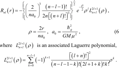
particle from the gravitational center. From quantum theory, on condition of E0, the normalized radial function of Equation (5) in spherical coordinate is
1
3 2
2 1 2 3 0
1 ! 2
2 !
l l
nl n l
n l
R r e L
na n n l
,
0 2r na
,
2
0 2
g a
GM
, (6)
where 2 1l
n lL is an associated Laguerre polynomial,
2 1
1 2 1
0
! 1
1 ! 2 1 ! ! n l
k
l k
n l
k
l n L
n l k l k k
.The allowed values of quantum numbers are
1, 2,3,
n and l0,1, 2n1. The “Bohr radius”
0
a is consistent with Equation (4). According to the shape and the initial revolving angular momentum of ob-served proto-planetary nebula disks, most of the nebular particles should be in states of the azimuthal quantum number ml = l, in which the particles revolve in the same direction around the equatorial plane of the system. The numerical simulation shows that all particles in these states form a gas disk similar to the observed nebular disk. The key question is what particles have affected the formation of planets. Though the old quantum model is rough, it still indicates some valuable information: the formation of the distances of inner and outer proto-plan-ets might be the result of the different distribution of hydrogen and helium particles. It is known that the mass of the proto-solar nebula is mostly made of hydrogen (71%) and helium (27%) gases, with tiny traces of other chemical elements and tiny dust particles. Therefore, hydrogen and helium, the most abundant gas particles, will be given the special attention.
Based on the Boltzmann equiprobability principle, we can assume that the particles distribute in each of the states described by above quantum number with equal probability. Since radial probability density of particles is rRnl
r 2, which can affect planetary distances, if the number of particles in every state is N, the radial mass density of some kind of particle with the mass in all these states can be written as
2. nl
n l
m r N
rR r . (7)Analytical expression of m(r) is very complicated, so the numerical calculating is adopted. It can provide a clear nature of the radial mass density. In calculation, the unit of distance is a0 of hydrogen atom, and N is an
appropriate constant due to the unimportance of its ab-solute magnitude. Though n may be all integers, nu-merical experiments show that when n20, the
in-crease of n has almost no influence on the characteristic of m(r) curve used in this paper. Here the maximum of n
is set at 30 for accuracy. The numerical experiments also show that only when l is all the allowed values, the regular fluctuation of the m(r) curve can appear. In this case, the spatial periods of the fluctuation correspond to the spacing of planets or satellites of the solar system.
4. Planetary Distances
4.1. Correspondences between Planetary Distances and m(r)
This model is first applied to the planets of the solar sys-tem. Based on the phenomena and analysis in the above sections, H, H2 and He, the most abundant particles in
nebular disk, are chosen as the investigated objects. The plots of m(r) are shown in Figure 1, where the a0 of
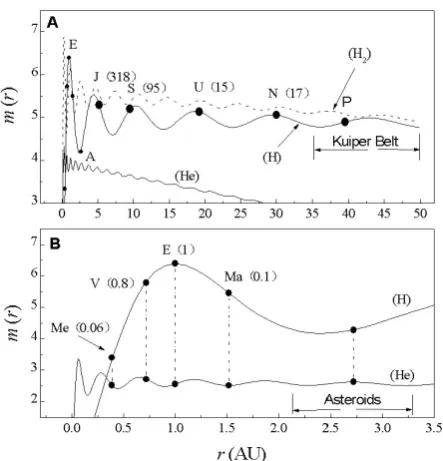
the H atom is set as 1 AU, and the ratios of the m(r) val-ues for the three curves have no real significance. The curves in Figure 1 have the following properties: 1) The
wave amplitudesof m(r) values is decreasing but wave-lengths increasing with the distance r. 2) The wave cy-cles of H curve from the first to the sixth correspond to the terrestrial planets, Jupiter, Saturn, Uranus, and Kui-per belt, respectively. 3) Six cycles of the He curve are included within the first cycle of the H curve, and the wave cycles of He curve from the second to the fifth re-spectively correspond to the Mercury, Venus, Earth and Mars, while the mean distance of asteroids belt is just at the sixth He wave crest but H wave trough.
There is no good correspondence between the wave cycles of the H2 curve and the planets, so we will not pay
any more attention to it in the following discussions. But it should be noticed that the wave crests of H curve from the first to the fifth overlap with H2 cure crests, and these
are the places that large planets exist. There is no large planet in the overlapping position of the sixth crest of H curve and the trough of the H2 curve, Kuiper belt exist
right there.
It is noticeable that the positions of planets are not ex-actly consistent with the wave crests of the m(r) curves of H or He, especially in terrestrial planets. These devia-tions are actually reasonable, which will be further spe-cially explained.
4.2. Significance of the Correspondences
[image:3.595.58.284.124.262.2]the wave crests of the m(r) curve. This means that the formation of proto-planets is the easiest at these radial density peaks. In the terrestrial region, the oscillation of radial density of helium particles is comparatively obvi-ous, i.e., the action of the potential wells of helium is stronger than that of other kinds of particles. Therefore, the particles can be aggregated more easily in these re-gions to form the proto-planets. This is just the reason why the terrestrial planets correspond to the m(r) waves of He. But the influence of the hydrogen particles is also important on the formation of the terrestrial planets, be-cause the largest gravity potential well be-caused by the first peak of the H curve lies in the middle of the terrestrial region, and it might cause the planetesimals or embryo in the region to move towards it during their growth. This can explain why the terrestrial planets all deviate from the He curve peaks, where planets should lie on, towards the first peak of the H curve. In the giant planet region, the oscillation amplitude of the He curve becomes much smaller, and the potential wells correspond to wave crests of the H curve act as the local gravity center. Therefore there exists a good correspondence between the giant planets and the m(r) peak of H.
From modern hypothesis on planetary formation [26,27], giant planets are formed because of the gravita-tional instability of gas in the accretion disk around young star, and terrestrial planets are formed by continuous col-lision and accumulation of larger planetesimals and planetary embryos. If it is true, the gravitational instabil-ity could be caused by the gravitational potential wells in the gas disk, and larger planetesimals and planetary em-bryos should be firstly formed nearby the potential wells. Actually, the quantum-like model can give the planetary formation mechanism a convincing support. From Figure 1, it can be seen that there are higher frequency and
greater intensity radial density wave of heavier elements in terrestrial region in comparison with giant planets re-gion. Accordingly, it can be speculated that: 1) Formation of planetesimals is easier, and the number is larger in ter-restrial region than in outer solar system. So the collision probability of planetesimals is larger, and the planetary embryos form easily and grow quickly at the wave crests of He. 2) In giant planets region, for the lack of heavier particles and the weakness of the fluctuation of their den-sity, the formation of planetesimals is more difficult. But because of the strong fluctuations of the radial density of hydrogen gas, the proto-planets are most possibly formed because of gravitational instability of the gas.
4.3. Signification of the Deviation
The deviation of the planetary positions will be discussed here. The locations of curve crests are about a0, 4.4a0, 10.3a0, 18.6a0, 29.5a0, 42.9a0, etc, where a0is equal
to 1 AU for H, and about 1/16 AU for He. Figure 1 (b)
displays the obvious deviation of the position of each terrestrial planet from the corresponding wave crest of He curve towards the first crest of H curve. It is worth notic-ing that the planetary deviation degree is roughly related to the slope of the H curve at the planetary corresponding position, and larger deviation corresponds to larger slope in either side of the crest of H. For example, the deviation of the Mercury is larger than that of the Venus in inner side of the H wave crest, while the deviation of the Mars is larger than that of the Earth in outer side. Since the sixth crest of the He curve is near the minimum point of H curve, where the slope is the smallest, the deviation of the asteroids from the He crest is also the smallest. If the matter distribution of the proto-solar system is surely similar to that in Figure 1, these deviations are reasonable.
As explained above, the formation of the terrestrial planetary positions depends not only on the distribution of helium, but also on that of hydrogen. If an embryo formed at the wave crest of He, it should shift from the crest towards the location with larger density of hydrogen in later accretion process. Besides, other mechanisms, such as their mutual gravitation, can also cause them to congregate. So we can speculate that if there is no strong tidal force from the Sun and Jupiter, a giant planet might be formed. Since the distribution of He atoms and other heavier particles lean to the interior of nebula disk, the position of this aborted giant planet should lie at the first crest of the H curve but deviate a little towards the Sun,
i.e., its distance from the Sun should be less than 1 AU. Such giant planets are possible in extrasolar systems.
The deviation of the Jupiter and Saturn shown in Fig-ure 1(a) can be explained by resonance mechanism. The
resonance can cause changes of some planetary positions in later evolvement [28]. Among all giant planets, since Jupiter and Saturn both have the largest mass and the shortest distance between them, their strong mutual at-traction can easily draw themselves close to each other. It is known that the mean-motion resonance of 5:2 exists in the Jupiter-Saturn system. If the mass ratio of the Jupiter to Saturn remains a constant in evolvement, and the initial distances were 4.4 AU for the Jupiter and 10.3 AU for the Saturn, the ratio of the initial angular momentum of the Jupiter-Saturn system to modern that, 10.2/10.7, can be obtained. Obviously, the ratio approximately obeys the conservation law of angular momentum. The increase of 5% of modern angular momentum may be explained by the action of the solar wind or the other mechanism.
5. Planetary Masses
Another interesting phenomenon in Figure 1 is the
shown in Figure 2, where the height of vertical bar
represents the mass of the planet. Apparently, except the Neptune, two corresponding relations appear in two sets of planets respectively. This correlation can be under-stood easily because hydrogen is the most abundant component of the solar system, and the final mass of planet should mainly depend on the radial density and the total mass of hydrogen in the region of planet formed. The larger radial density can cause the proto-planet to form earlier and grow more quickly, and so become a larger mass planet. The mass of the Neptune is slightly larger than Uranus, which is an intelligible exception. The Neptune is the outermost giant planet, and its region of provisioning material can be extended outwards into the Kuiper belt, so its mass can become larger.
6. Asteroid Belt and Kuiper Belt
An interesting coincidence between the asteroid belt and Kuiper belt can be seen from Figure 1. Asteroid belt and
Kuiper belt respectively correspond to the sixth wave cycle of the He curve and the H curve, and the asteroid belt lies at the overlapping region of the crest of He with the trough of the H curve, while the Kuiper belt lies at the overlapping region of the crest of H with the trough of the H2 curve. This means that the material density in
the two regions is too few to the formation of the planets. This might be one of the reasons why there are no large planets in these positions.
In Figure 1(b), the distance between the two troughs
of the sixth wave of He curve is 2.2-3.1 AU. It is close to the width of about 2.1-3.3 AU of the asteroid belt shown in Figure 3, which is prepared on 2011 March 20 by
IAU Minor Planet Center (MPC) [29].
The position of the sixth crest of the He curve is 2.7 AU, which is just the radial geometrical center of the asteroid belt.
Similarly, from Figure 1(a), the distance between the
two troughs of the sixth wave of the H curve is 36-50 AU, which is consistent with the current observed range of Transneptunian Objects (TNOs), also called Kuiper belt objects (KBOs). Figure 4 is the statistics for
popula-tion of 1163 TNOs promulgated by MPC in 2011 March [29]. Their orbital semi-major axis distribute between 35 - 50 AU, which is called the main Kuiper belt [30]. This population pattern has not changed since 2002 [22], al-though the number of observed objects has increased twice. In addition, we do not worry about the effect of Centanurs and SKBOs (scattered Kuiper belt objects), whose number is smaller, and the most of them distribute inside the Neptune orbit and outside 50AU respectively. They have properties different from the TNOs, and their population is not innate. So they are not considered here.
Figure 1. The m(r) curves of particles and planetary dis-tances. The solid lines are m(r) curves of H and He particles, the dashed is one of H2, the filled circles represent the planetary positions, and the numbers in brackets are planetary masses.
0 5 10 15 20 25 30 35
0 1 2 3 4 5 6 7
B
m
(
r
)
5.06 5.15
5.27 5.54
Uranus (15)
Neptune (17) Saturn
(95) Jupiter (318)
r (AU)
0.0 0.2 0.4 0.6 0.8 1.0 1.2 1.4 1.6 1.8 2.0 0
1 2 3 4 5 6 7
A
Mars (0.1) Earth
(1.0) Venus (0.8)
Mercury (0.06)
5.45 6.39
5.83
3.33
Figure 2. Relation between the planetary mass and the ra-dial density of H.
[image:5.595.312.534.84.315.2] [image:5.595.316.534.403.604.2]resonance region of Neptune or were scattered into the other space. There is an absence of objects between the resonance belt of 3:2 and 43 AU. The major part of these absent objects might have been removed. This characteris-tic of distribution of KBOs shown in Figure 4 cannot be
completely illustrated by the mechanism of the Neptune resonance [31], unless the distribution of the initial mate-rial is the same as the m(r) curve shown in Figure 1.
Zuo et al. have simulated the evolution of the Kuiper belt by the time regression method, and have obtained the expected results that before 4.5 × 10⁸ yrs the
distribu-tion pattern of the KBOs is almost same as theory using
m(r) curve [32]. We can predict that despite the increas-ing of number of objects, the center of the Kuiper Belt should remain at about 43 AU, which is the wave crest of the m(r) curve.
[image:6.595.57.284.316.499.2]Since Pluto is only the largest object lying in 3:2 reso-nance in the Kuiper belt, and have lost its large planetary status, no attention will be paid to it in this paper.
Figure 3. Distribution of the minor planets.
32 34 36 38 40 42 44 46 48 50 52
0 50 100 150 200 250 300
3:2 resonance
1163 KBOs
N
u
m
ber
of
O
b
je
c
ts
[image:6.595.63.284.529.714.2]Semimajor axis (AU)
Figure 4. Distribution of KBOs.
7. Satellites and Ring System
The model can also be applied to explain the regular sat-ellites and ring system of planets. Numerical fitting shows that if the “Bohr radius” of H particle in planetary gravitational field is 95.2 10 km3
J
a for Jupiter, 3
S 28.4 10 km
a for Saturn, and 3 U 4.4 10 km
a
for Uranus, many corresponding relations in Figure 5
can be discovered.
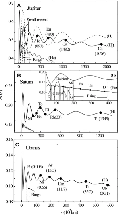
Figure 5(a) shows the relation between the regular
satellites of Jupiter and the distribution of the materials in the model. The positions of the four Galilean satellites correspond to the four wave crests of H2 curve
respec-tively, and the three larger satellites, Io, Ganymede, and Callisto, just locate at the superposition region of the wave crests of H and H2 curves. The Europa with smaller
mass is at the crest of H2 curve but at the trough of H
curve. Besides, most of the inner small moons of Jupiter also lie near crests of H2 curve. This means that the role
of the hydrogen molecules in the formation of satellites might be more important than that of hydrogen atoms. The Jupiter has a ring system including a halo (89.4 - 123.0 × 10³ km), the main (123.0 - 128.9 × 10³ km) and a
gossamer ring(128.9 - 242.0 × 10³ km) [33]. The brighter
halo and the main ring just occupy one wave of He curve, and the end of the gossamer ring is at the overlapping region of two trough of H and He waves.
The chief graph in Figure 5(b) mainly illustrates the
relation between the distribution of H atoms and posi-tions of six large satellites of Saturn. Two largest satel-lites, Titan and Rhea, accurately lay at the wave crests of H curve. The distribution of the other four smaller satel-lites, Mimas, Enceladus, Tethys, and Dione is very simi-lar to that of the terrestrial planets. The inset graph shows clearly that the four satellites respectively correspond to the four wave cycles of He curve and are included in a wave cycle of H curve, and Enceladus, Tethys, and Dione all slide down the corresponding wave crests of He curve and are close to the crests of H curve except Mimas being at the trough of H curve.
It is impressive that the distribution of rings and the most of the moonlets of Saturn also accord with the fluc-tuation of He curve. The D ring (66.9 × 10³ - 74.7 × 10³
km) and C ring (74.7 × 10³ - 92.0 × 10³ km) occupy one
wave cycle of He curve, B ring (92.0 × 10³ - 117.5 × 10³ km) just takes up the next one, the narrow F ring (140 × 103 km) and nearby five moonlets are at the He wave crest
following B ring, while the French division (90 × 103- 92
× 103 km) and Cassini division (118 × 103 - 122 × 103 km)
are exactly in the two troughs of wave corresponding B ring respectively. Another coincidence is that if E ring is really defined observationally to lie in the region about 3.3 - 6.5 Saturn radii [34], which is 60 × 103 km, it will be
cy-cle of H curve, from about 200 × 103 km to 390 × 103 km. Figure 5(c) displays that six larger satellites of Uranus
correspond to the wave crests of H curve well, and the ring of Uranus is just at a wave crest.
From the above analysis we believe that the formation of the three planet systems is related to the distribution of initial hydrogen. The molecule composition of hydrogen around the Jupiter is more than that of the Saturn and Uranus due to larger gas density caused by large mass of the Jupiter, so the correspondences of them with H2 or H
curve are reasonable. In addition, there is an absent object in every curve in Figure 5, while the masses of satellites
near these spaces are all the largest, such as Ganymede of Jupiter, Titan of Saturn, and Titania of Uranus. It can be assumed that the materials here have been captured by these largest satellites for other mechanism.
0 500 1000 1500 2000 0.4 0.5 0.6 0.7 Rings A m ( r ) (He) Jupiter
(H2) (H) Ca (1076) Ga (1482) Eu (480) Io (893) Small moons
100 200 300 400 0.10
0.15 0.20
r (103km) E ring G D Di Te En Mi F Division A B C (He) (H)
0 100 200 300 400 500 600 0.08 0.10 0.12 0.14 0.16 C (H) Ob (30.1) Ti (35.2) Uranus Um (11.7) Ar (13.5) Mi (0.66) Pu(0.005) Rings
0 300 600 900 1200 0.15 0.20 0.25 Saturn B (H) En Mi Te Di
[image:7.595.70.278.290.664.2]Rh(23) Ti (1345)
Figure 5. The correspondence of m(r) curves with the satel-lites and rings of planets. Here, every satellite is marked with the first two letters of its name. The dashed vertical lines give the locations of the rings. The numbers in the brackets are the mass of the satellites (in unit 1020 kg).
8. Energy and Angular Momentum of the
Planetary Region
Whether the original nebular radial density really follows
m(r) curves, there are further evidence according to the comparison of the energy and angular momentum in plan-ets districts. Considering interaction between planplan-ets dur-ing their formation and growth, the system is divided into four regions as given in Table 1, which adopts Dai me-
thod [35]. The inner boundary of the terrestrial region is the trough of the helium m(r) curve. Based on quantum mechanics, the energy of a particle with mass in n
state is 2
0
2 n
E GM n a . From Equation (7), the ra- dial number density of a certain particle is
2. nl
n l
N
rR r . The total energy of particles in a thin spherical shell with thickness dr is
2,
d n nl n l
EN
E rR r r. If there are two kinds of particles, H and He atoms, the energy density in each of the regions can be expressed asm Ei mi
, where Ei and mi are the total en-ergy and the total mass of a certain kind of particles re-spectively, and they can be written as
2 1 2 2 , 0 d 2 r i ii i r nl
n l i GM
E N rR r r
n a
, (8)
2 1 2 , d r ii i i r nl n l
m N
rR r r, (9)where r1 and r2are the inner and the outer radii of the
region respectively, and i
nlR r represents the radial wave function of a certain kind of particles. Based on the above two equations, the energy carried by the unit mass of the nebula (called energy density) in each of the four regions can be calculated by letting the ratio of the total mass iNi of H and He in the solar system be 71: 27, and the unknown Ni can be eliminated. The calculated values of m in unit (GM/ 2a0 H ) are given in Table 1, where a0 H is “Bohr radius” of H particle. The
ac-tual energy of planets can be calculated by GMm/ 2a, where m and a are planetary mass and semi-major axis respectively. The energy density p of every planetary district is also given in Table 1 for comparison. It is
clear that the data of the model and the observation fit well.
The similar method is used to calculate the angular momentum of the unit mass nebula (called angular mo-
Table 1. The comparison of the angular momentum and energy.
[image:7.595.308.538.667.722.2]mentum density). z axis component of the angular mo-mentum of a particle in l states is written as Lz lg. In each region, the total angular momentum of a certain kind of particles can be written as
2 1
2
,
d
r i
zi i g r nl
n l
J N
l rR r r. (10)The angular momentum density in each region is cal-culated by jm
Jzi
mi . Since g is unknown, we take the value of the Uranus region as unit. The ap-proximate equation calculating of the angular momentum of the planet is
1 2
p
J m G M m a e , where e is the orbital eccentricity. The angular momentum density of a planet is jpJp/m, the unit is that of the Uranus. The calculated values of nebular and the actual values of the planets in each region are listed in Table 1. It is also
seen that the model is consistent with observation, except the terrestrial region.
In conclusion, Table 1 shows a strong consistency
be-tween the theory and the observation in three giant planets regions, but the deviations in the terrestrial region are lar-ger, especially for the angular momentum. Actually, this is reasonable as a result when most of the original gas mate-rials have escaped from the terrestrial region. There are two reasons for the increase in the angular momentum of the unit mass of planets: 1) planets had captured particles with large angular momentum, 2) planets formation region had lost the materials with smaller angular momentum. In the terrestrial region,the maximum amount of the pri-mordial materials is H particles which are in l0 state with zero angular momentum, and the next is smaller ratio of helium and other heavier particles being in any possible
l state with larger angular momentum. During the earlier period of the Sun formation, the solar wind is very weak, so that H particles with zero angular momentum can be easily captured by the Sun. In the later stage, the strong solar wind takes away the most of H particles again and left some angular momentum in the collision with planets materials. Both the mechanisms can all make terrestrial region lose a lot of mass carrying small amount of angular momentum. Even the angular momentum taken away by solar wind might be smaller than what is brought in. As a result, the angular momentum of the unit mass of planets in the terrestrial region is increased. We can make a simple estimation. Let the original total mass of terrestrial region be m, the lost mass with zero angular momentum be x m , and
m xm
is planetary mass. Since the ratio of origi-nal 0.074 and modern 0.214 (see Table 1), the totalorigi-nal angular momentum is 0.074m 0.214
m xm
. The ratio of lost mass can be obtained as x65.4%, which is reasonable. In addition, since the energy of the particle is proportional to the mass, the energy will natu-rally decreases with the decrease of the mass, and the ratioof energy and mass will be a constant approximately. So there is only small deviation of energy of the unit mass in the terrestrial region.
In this section, the planetary rotation has not been mentioned because the rotation energy and angular mo-mentum are much smaller than the orbital ones.
9. Conclusions and Discussion
To conclude, in the study of the basic problems of the solar system origin, the quantum-like model described in this paper would be more efficient than others. Many correspondences mentioned above are neither far-fetched and obscure, nor haphazard coincidence. It is possible that an unknown truth will be revealed. Above research can inspire us to make the following hypotheses:
1) The chaos behavior of nebular particles in gravita-tional field can be described by the wave function satis-fying the Schrödinger equation when we replace the
with g.
2) The distribution of H and He particles might play the important roles in formation of the planets. Waves of radial density of H atoms formed a series of largest rings, and the terrestrial planets, Jupiter, Saturn, Uranus, Nep-tune, as well as the Kuiper belt formed in these rings respectively. The rings of He atoms are thinner than those of H. The first H ring covers four He rings, where the original terrestrial planets formed respectively, but due to the influence of H ring, they have shifted toward the center of H ring.
3) The distribution of heavier elements is closer to the Sun than hydrogen and helium. The rings made from heavier particles are thinner and denser than those of He. A ring of He contains tens or hundreds of thin rings made of heavier particles, and the thin ring contains the thinner rings, which like the form of the observed rings of Saturn. With the decrease of the distance from the Sun, rings be-come denser and thinner gradually. They might be impor-tant for the formation of planetesimals. Due to more heavy elements and planetesimals in the terrestrial region than other regions, the formation of terrestrial planets is easier. As to the giant planets region, as the lack of heavy ele-ments and planetesimals, the formation of proto-planets can only depend on the gravitational instability of gas.
the mass of Neptune is still larger than Uranus. Due to strong solar wind and the strong tidal forces from the Sun and Jupiter, the terrestrial region cannot form a giant planet.
5) The formation mechanism of satellites differs from that of planets. The regular satellites might form in a circumplanetary accretion disk produced by a slow in-flow of gas and solids during the end of the planet for-mation [36]. The gas should form an envelope, in which the gas matter distribution is the same as shown in Fig-ure 5. When the planetesimals in exterior space fall into
the envelope, they should be likely to stay nearby the radial density crest of gas by the stickiness of gas, and finally form satellites. In this way, the mass of outer sat-ellites is naturally greater than inner ones.
6) Due to the special position in H wave, the rotation speeds of Mercury and Venus gradually slow down by asymmetric viscous resistance. The resistance is so ef-fective that the rotation direction of Venus is reversed. The results have already published [23], we did not dis-cussed in this paper.
This paper shows a perfect structure of the solar sys-tem, which can be divided into two symmetrical quantum groups: 1) the Jupiter, Saturn, Uranus, Neptune and the Kuiper belt; 2) the Mercury, Venus, Earth, Mars and the asteroid belt. Their quantum orders are all described as
2,3, 4,5,6
n , and the width of the planetary districts of the giant planets group is 16 times that of the terrestrial group. This ratio is that of the atom mass square of he-lium and hydrogen, which are the main particles in primitive nebula of the solar system. According to these facts, it can be predicted that the structure of the solar system has been basically fixed, and it is impossible to find any major planets inside the orbit of Mercury and outside the Kuiper belt, but the minor planets or dwarf planets similar to Pluto may be found inside or outside the Kuiper belt.
In addition, this paper provides an initial distribution state of the solar nebula, using the initial conditions, the formation of planets and satellites can be simulated, al-though the workload is quite large.
10. Acknowledgements
The author would like to thank Prof. Chuanfu Cheng, Prof. Qingtian Meng for their help in English writing of this paper, and would also thank the reviewers whose comments have caused great improvement of this paper. The author is grateful to David Jewitt for the data from his Internet Station. At last, the author would express her thanks to The SAO/NASA Astrophysics Data System for the consulting on references.
11. References
[1] M. M. Nieto, “Conclusions about the Titius Bode Law of Planetary Distances,” Astronomy and Astrophysics, Vol. 8, 1970, pp. 105-111.
[2] L. Basano and D. W. Hughes, “A Modified Titius-Bode Law for Planetary Orbits,” Nuovo Cimento C, Vol. 2C, No. 5, 1979, pp. 505-510. doi:10.1007/BF02557750 [3] E. Badolati, “A Supposed New Law for Planetary
Dis-tances,” Moon and the Planets, Vol. 26, May 1982, pp. 339-341. doi:10.1007/BF00928016
[4] V. Pletser, “Exponential Distance Laws for Satellite Sys-tems,” Earth, Moon, and Planets, Vol. 36, 1986, pp. 193- 210. doi:10.1007/BF00055159
[5] R. Neuhaeuser and J. V. Feitzinger, “A Generalized Dis-tance Formula for Planetary and Satellite Systems,” As-tronomy and Astrophysics, Vol. 170, No. 1, 1986, pp. 174-178.
[6] P. Lynch, “On the Significance of the Titius-Bode Law for the Distribution of the Planets,” Monthly Notice of the Royal Astronomical Society, Vol. 341, No. 4, 2003, pp. 1174-1178. doi:10.1046/j.1365-8711.2003.06492.x [7] L. Neslušan, “The Significance of the Titius-Bode Law
and the Peculiar Location of the Earth’s Orbit,” Monthly Notice of the Royal Astronomical Society, Vol. 351,No. 1, 2004, pp. 133-136.
[8] G. Gladyshev, “The Physicochemical Mechanisms of the Formation of Planetary Systems,” Moon and the Planets, Vol. 18, April 1978, pp. 217-222.
doi:10.1007/BF00896744
[9] J. J. Rawal, “Contraction of the Solar Nebula,” Earth, Moon, and Planets, Vol. 31, October 1984, pp. 175-182. doi:10.1007/BF00055528
[10] X. Q. Li, Q. B. Li and H. Zhang, “Self-similar Collapse in Nebular Disk and the Titius-Bode Law,” Astronomy and Astrophysics, Vol. 304, 1995, pp. 617-621.
[11] F. Graner and B. Dubrulle, “Titius-Bode Laws in the Solar System 1: Scale Invariance Explains Everything,” Astronomy and Astrophysics, Vol. 282, No. 1, 1994, pp. 262-268.
[12] R. Louise, “A Postulate Leading to the Titius-Bode Law,” Moon and the Planets, Vol. 26, February 1982, pp. 93-96. doi:10.1007/BF00941371
[13] R. Wayte, “Quantisation in Stable Gravitational Sys-tems,” Moon and the Planets, Vol. 26, February 1982, pp. 11-32. doi:10.1007/BF00941366
[14] R. Louise, “The Titius-Bode Law and the Wave Formal-ism,” Moon and the Planets, Vol. 26, June 1982, pp. 389- 398. doi:10.1007/BF00941641
[15] R. Louise, “Quantum Formalism in Gravitation Quantita-tive Application to the Titius-Bode Law,” Moon and the Planets, Vol. 27, August 1982, pp. 59-63.
doi:10.1007/BF00941557
[17] Q. X. Nie, “Simulated Quantum Theory for Seeking the Mystery of Regularity of Planetary Distances,” Acta As-tronomica Sinica, Vol. 34, No. 3, 1993, pp. 333-340. [18] K. U. Lu, “Mathematical Investigation of Bode’s Law
and Quantilization of Gravity,” Astrophysics and Space Science, Vol. 225, No. 2, 1995, pp. 227-235.
doi:10.1007/BF00613237
[19] B. E. Yang, “Introduction to Quantum Theory on Planets and Satellites (in Chinese),” Dalian University of Tech-nology Press, Dalian, 1996, pp. 27-32.
[20] A. G. Agnese and R. Festa, “Clues to Discretization on the Cosmic Scale,” Physics Letters A, Vol. 227, No. 3-4, 1997, pp. 165-171. doi:10.1016/S0375-9601(97)00007-8 [21] L. Nottale, G. Schumacher and J. Gay, “Scale Relativity
and Quantization of the Solar System,” Astronomy and Astrophysics, Vol. 322, 1997, pp. 1018-1025.
[22] Q. X. Nie, “The Characteristics of Orbital Distribution of Kuiper Belt Objects,” Chinese Astronomy and Astro-physics, Vol. 27, No. 1, 2003, pp. 94-98.
[23] Q. X. Nie, Cuan Li and F.-S. Liu, “Effect of Interplane-tary Matter on the Spin Evolutions of Venus and Mer-cury,” International Journal of Astronomy and Astro-physics, Vol. 1, No. 1, 2011, pp. 1-5.
doi:10.4236/ijaa.2011.11001
[24] G. G. Comisar, “Brownian-Motion Model of Nonrelativis-tic Quantum Mechanics,” Physical Review, Vol. 138, No. 5B, 1965, pp. 1332-1337.
doi:10.1103/PhysRev.138.B1332
[25] E. Nelson, “Derivation of the Schrödinger Equation from Newtonian Mechanics,” Physical Review, Vol. 150, No. 4, 1966, pp. 1079-1085. doi:10.1103/PhysRev.150.1079 [26] A. P. Boss, “Astrometric Signatures of Giant-planet
For-mation,” Nature, Vol. 393, No. 6681, 1998, pp. 141-143.
doi:10.1038/30177
[27] A. P. Boss, “Rapid Formation of Outer Giant Planets by Disk Instability,” The Astrophysical Journal, Vol. 599, No. 1, 2003, pp. 577-581. doi:10.1086/379163
[28] N. Murray and M. Holman, “The Origin of Chaos in the Outer Solar System,” Science, Vol. 283, No. 5409, 1999, pp. 1877.doi:10.1126/science.283.5409.1877
[29] D. Jewitt, “Kuiper Belt,” 2011.
http://www2.ess.ucla. edu/~jewitt/kb.html
[30] J. X. Luu and D. C. Jewitt, “Kuiper Belt Objects: Relics from the Accretion Disk of the Sun,” The Annual Review of Astronomy and Astrophysics, Vol. 40, 2002, pp. 63- 101. doi:10.1146/annurev.astro.40.060401.093818 [31] R. Malhotra, “The Origin of Pluto’s Orbit: Implications for
the Solar System beyond Neptune,” Astronomical Journal, Vol. 110, 1995, pp. 420-429. doi:10.1086/117532
[32] Q. L. Zuo, Qing-xiang Nie, et al., “Simulations for Origi-nal Distribution of KBOs,” Acta Astronomica Sinica., Vol. 49, No. 4, 2008, pp. 413-418
[33] C. D. Murray and S. F. Dermott “Solar System Dynam-ics,” Cambridge University Press, Cambridge, 1999, pp. 532-533.
[34] J. A. van Allen, et al., “Saturn’s Magnetosphere, Rings, and Inner Satellites,” Science, Vol. 207, January 25 1980, pp. 415-421. doi:10.1126/science.207.4429.415
[35] W. S. Dai, “An Interpretation of the Titius-Bode Law,” Acta Astronomica Sinica, Vol. 16, No. 2, 1975, pp. 123- 130.
[36] R. M. Canup and W. R. Ward, “Formation of the Galilean Satellites: Conditions of Accretion,” The Astronomical Journal, Vol. 124, No. 6, 2002, pp. 3404-3423.