The SAMI Galaxy Survey : Data Release Two with absorption line physics value added products

The SAMI Galaxy Survey: Data Release Two with absorption-line

physics value-added products

Nicholas Scott ,

Jesse van de Sande,

Scott M. Croom ,

Brent Groves,

Matt S. Owers,

Henry Poetrodjojo,

Francesco D’Eugenio,

Anne M. Medling,

†

Dilyar Barat,

Tania M. Barone,

Joss Bland-Hawthorn,

Sarah Brough ,

Julia Bryant,

Luca Cortese ,

Caroline Foster ,

Andrew W. Green ,

Sree Oh,

Matthew Colless ,

Michael J. Drinkwater ,

Simon P. Driver,

Michael Goodwin,

Madusha L. P. Gunawardhana,

Christoph Federrath,

Lloyd Harischandra,

Yifei Jin,

J. S. Lawrence,

Nuria P. Lorente,

Elizabeth Mannering,

Simon O’Toole,

Samuel N. Richards ,

Sebastian F. Sanchez,

Adam L. Schaefer,

Katrina Sealey,

Rob Sharp,

Sarah M. Sweet ,

Dan S. Taranu

and

Mathew Varidel

Affiliations are listed at the end of the paper

Accepted 2018 August 27. Received 2018 August 27; in original form 2018 July 2

A B S T R A C T

We present the second major release of data from the Sydney – Australian Astronomical Observatory Multi-Object Integral Field Spectrograph (SAMI) Galaxy Survey. Data Release Two includes data for 1559 galaxies, about 50 per cent of the full survey. Galaxies included have a redshift range 0.004< z <0.113 and a large stellar mass range 7.5<log (M/M)<

11.6. The core data for each galaxy consist of two primary spectral cubes covering the blue and red optical wavelength ranges. For each primary cube, we also provide three spatially binned spectral cubes and a set of standardized aperture spectra. For each core data product, we provide a set of value-added data products. This includes all emission line value-added products from Data Release One, expanded to the larger sample. In addition, we include stellar kinematic and stellar population value-added products derived from absorption line measurements. The data are provided online through Australian Astronomical Optics’ Data Central. We illustrate the potential of this release by presenting the distribution of∼350 000 stellar velocity dispersion measurements from individual spaxels as a function ofR/Re, divided

in four galaxy mass bins. In the highest stellar mass bin [log (M/M)>11], the velocity

dispersion strongly increases towards the centre, whereas below log (M/M)<10 we find

no evidence for a clear increase in the central velocity dispersion. This suggests a transition mass around log (M/M)∼10 for galaxies with or without a dispersion-dominated bulge.

Key words: galaxies: abundances – galaxies: general – galaxies: kinematics and dynamics – galaxies: star formation – galaxies: stellar content – astronomical data bases: surveys.

_{E-mail:[email protected]}

†Hubble Fellow.

1 I N T R O D U C T I O N

Galaxies are composed of multiple distinct components, such as thin and thick discs, bulge, bar(s), spiral arms, ring(s), and many others. As well as having different spatial structures, these components can also differ in terms of their kinematics and their compositions,

2018 The Author(s)

either narrowly in terms of differing chemistry, or more broadly into stellar, gaseous, and dark matter. Determining how these distinct components interact and change over time is critical to a deeper understanding of galaxy evolution (e.g. Mo, van den Bosch & White

2010).

Spatially resolving galaxiesis essential to understand the differ-ent compondiffer-ents. While imaging studies, particularly multiwave-length imaging, can begin to disentangle these components, access to kinematic and chemical separation is largely unavailable. Spa-tially resolved spectroscopy is ideally suited to this task, as the simultaneous separation of the observed light, both spectrally and spatially, provides the most detailed dissection of the internal

struc-ture of galaxies currently available (e.g. Cappellari2016).

The challenge of spatially resolved spectroscopy is that spread-ing the light out both spatially and spectrally drastically reduces the signal-to-noise ratio (S/N) per resolving element. This limitation has restricted initial work in this area to relatively small samples of objects, or to specific classes of object that are more easily ob-served. While these kinds of studies have been very successful in addressing the role of specific physical processes that shape galax-ies, a broader view is required to develop a holistic understanding of galaxy evolution.

Galaxies are very diverse, and the physical processes involved in galaxy evolution are many and varied. To fully understand the primary drivers of galaxy evolution, one requires large samples that encompass the complete diversity of the galaxy population. This can be achieved with spatially resolved spectroscopy by either investing large amounts of telescope time with a single-object

in-strument, e.g. surveys withN>250, ATLAS3D_{(Cappellari et al.}

2011), and CALIFA (S´anchez et al.2012), or through the use of a

multiplexed integral field spectrograph (IFS), such as the Sydney – Australian Astronomical Observatory Multi-Object Integral Field

Spectrograph (SAMI; Croom et al.2012), MaNGA (Bundy et al.

2015), or KMOS (Wisnioski et al.2015; Stott et al.2016). Since

the beginning of this decade, large integral field spectroscopy sur-veys such as these have been assembling samples of hundreds or thousands of galaxies, allowing us to dissect, in detail, the entire population of local galaxies.

Green et al. (2018, SAMI Data Release One, hereafter DR1)

discussed the broad role integral field spectroscopy has played in furthering our understanding of galaxies. In the current release, we hope to push forward the exploration of new analyses that utilize the full power of combining emission, absorption, and dynamical measurements by providing extensive value-added data products.

In this paper, we present the second public release (DR2) of SAMI Galaxy Survey observations, including both fully processed spectral data cubes and a large array of derived science products that enable an extremely broad approach for studying galaxies. In Section 2 we briefly review the survey and instrument design and progress on observing and processing the data since DR1. In Section 3 we describe the galaxies presented in this sample. In Section 4 we describe the core data of this release, spatially resolved spectral cubes and additional spectral data derived from these cubes, and the quality of the data. In Section 5 we describe the emission line products included in this release, with a focus on changes since DR1, and in Section 6 we describe the new absorption line products being released for the first time. Finally, in Section 7 we describe how these data can be accessed through the Data Central web service and provide an example science use of these data to illustrate the potential power of this data release. Throughout this release, we

adopt the concordance cosmology: (, m, h)=(0.7,0.3,0.7)

(Hinshaw et al.2009).

2 T H E S A M I G A L A X Y S U RV E Y

The SAMI Galaxy Survey (Bryant et al.2015) is a spatially resolved

spectroscopic survey of a large sample of nearby (z0.1) galaxies,

conducted with the SAMI instrument (Croom et al.2012).

The SAMI instrument is a multi-object IFS mounted at the prime focus of the 3.9 m Anglo-Australian Telescope (AAT). SAMI uses 13 fused optical fibre bundles (hexabundles; Bland-Hawthorn et al.

2011; Bryant et al.2011, 2014) that can be deployed across a 1

deg diameter field of view. Each hexabundle consists of 61 closely packed optical fibres, where each fibre has a diameter of 1.6 arc-sec, resulting in an integral field unit (IFU) with a diameter of 15 arcsec and a fill factor of 75 per cent; 26 additional fibres provide simultaneous blank sky observations.

SAMI feeds the AAOmega optical spectrograph (Sharp et al.

2006). The SAMI Galaxy Survey makes use of the 580V and 1000R

gratings, with a dichroic to split the light at 5700 Å between the two spectrograph arms. The precise wavelength coverage and spectral

resolution of this instrumental set-up are given in Table1.

2.1 Survey sample and observing status

The selection of the SAMI Galaxy Survey sample is described in

detail in Bryant et al. (2015), with further details in Owers et al.

(2017). Here we briefly summarize the primary sample and describe

the status of secondary targets.

The SAMI Galaxy Survey sample consists of two separate but complementary samples with matched selection criteria; a SAMI– GAMA sample drawn from the Galaxy And Mass Assembly

(GAMA) survey (Driver et al.2011) and an additional cluster

sam-ple. The SAMI–GAMA sample consists of a series of volume-limited samples, where the stellar mass limit for each sample in-creases with redshift. Stellar masses are estimated from the

rest-frame i-band absolute magnitude andg− icolour by using the

colour–mass relation following the method of Taylor et al. (2011),

assuming a Chabrier (2003) stellar initial mass function (IMF)

and exponentially declining star formation histories. The SAMI–

GAMA sample is drawn from the three 4×12 deg fields of the

initial GAMA-I survey (Driver et al.2011). These regions include

galaxies in a range of environments, from isolated up to massive

groups, but do not contain any galaxy clusters within thez≤0.1

SAMI limit. To complete the environmental coverage, the SAMI Galaxy Survey includes an additional cluster sample, drawn from

eightz≤0.1 clusters, described in Owers et al. (2017). The same

stellar mass selection limits were applied to the cluster sample as

for the main sample. In practice, for the clusters withz <0.045 we

target cluster galaxies with log (M/M)>9.5, and for the clusters

with 0.045< z <0.06 we target cluster galaxies with log (M/M)

>10.0.

In addition, a sample of secondary target galaxies is defined by galaxies with slightly lower stellar mass cuts in each redshift bin,

along with high-mass [log (M/M) > 10.9] galaxies at slightly

higher redshift (0.095< z <0.115). The secondary targets were

observed when a hexabundle could not be allocated to a primary target. This became necessary as the completeness of the survey grew. In the final semester of observations an extra set of ancillary galaxies was needed to occupy all hexabundles. These were pri-marily drawn from GAMA galaxies that are in pairs or groups with SAMI galaxies but did not meet the stellar mass cuts of the original selection criteria. None of the ancillary targets are included in DR2. Survey observations began in 2013 March and were completed in 2018 May. There were a total of 250 observing nights, spread over 34

(λrange), central wavelength (λcentral), median FWHM of the best-fitting Gaussian to the spectral instrumental LSF

in Å, the standard deviation of this Gaussian in Å, the spectral resolution atλcentral(Rλ−central), the velocity resolution

(FWHM) in km s−1_{(v), and the dispersion resolution (1σ) in km s}−1_(σ).

Arm λrange(Å) λcentral(Å) FWHM (Å) σ(Å) Rλ−central v(km s−1) σ(km s−1)

Blue 3750–5750 4800 2.66+₋0_0..076₀₇₀ 1.13 1808 165.9 70.4 Red 6300–7400 6850 1.59+₋0_0..049₀₄₀ 0.68 4304 69.7 29.6

individual observing runs. At the completion of survey observing, just over 3000 total galaxies were observed. The primary sample was observed to a completeness of 80 and 84 per cent in the GAMA and cluster regions, respectively, with 1930 and 724 unique primary targets in those regions.

2.2 Data reduction

The reduction of SAMI data and the production of data cubes are

described fully in Allen et al. (2015) and Sharp et al. (2015). Here we

briefly summarize the process and in the following section describe in detail the changes since the previous release.

SAMI data reduction broadly falls into two phases: the extraction of row stacked spectra (RSS) from raw observations and the con-struction of data cubes from the RSS frames. The creation of RSS

frames is handled by the 2DFDR data reduction package.1_Cube

creation is carried out using the SAMIPYTHON package (Allen

et al.2014), and the entire process is automated using the ‘SAMI

Manager’, part of the SAMIPYTHONpackage.

Initial reduction consists of the standard steps of overscan sub-traction, spectral exsub-traction, flat-fielding, fibre throughput calibra-tion, wavelength calibracalibra-tion, and sky subtraction. These steps are

all accomplished with 2DFDR, and result in one RSS frame per

observation. Each RSS frame contains data for 12 galaxies and a single calibration star for secondary spectrophotometric calibration and telluric correction.

Relative and absolute flux calibration and telluric correction are

applied to each RSS frame using the SAMIPYTHONpackage. The

flux-calibrated RSS frames are combined into three-dimensional data cubes by resampling on to a regular grid. This combination includes dither registration and differential atmospheric refraction correction and an additional absolute flux calibration step. The result is a three-dimensional (two spatial and one spectral) data cube. Covariance between spaxels is calculated and stored within the

cubes in a compressed form (see Sharp et al.2015for details).

Binned cubes and aperture spectra are also produced at this stage (see Sections 4.2 and 4.3 for details).

2.2.1 Changes between DR1 and DR2

For this release, we use the SAMIPYTHONpackage snapshot

iden-tified asMERCURIALchangeset 17EBC0FF0A1C, and 2DFDR version

6.65. Several aspects of the data reduction have been improved be-tween these software versions and those used for DR1, which we

document in detail below. In addition, the SAMIPYTHONpackage

has experienced some quality-of-life improvements including op-timization of computationally intensive aspects of the package as

compiled C code, support forPYTHON3 compatibility, and increased

terminal feedback during data reduction. Three main aspects of the

1_{https://www.aao.gov.au/science/software/2dfdr}

data reduction have been improved for this release. They are as follows: extraction of spectra, flat-fielding, and wavelength calibra-tion.

Spectral extraction requires an accurate trace of the fibre locations across the detector. These traces (that we call a tram-line map) are derived from a calibration frame, and are based on Gaussian profile fits to each fibre in the spatial direction. This fit is repeated for each CCD column and the resulting fibre locations are then fitted with a smoothly varying function. For DR1 and earlier releases, this tram-line map was determined from dome flat calibrations taken as part of a standard science observation sequence. However, the dome

flat frames have relatively low counts below∼4000 Å, resulting in

higher uncertainties in the tram-line maps in the far blue. For DR2 we used twilight sky frames to derive tram-line maps, resulting

in more accurate traces below ∼4000 Å with improved spectral

extraction and reduced cross-talk between adjacent fibres. Where twilight sky observations are not available for a given field, we use twilights from different fields. To account for shifts between tram-line maps from different fields (and on occasion different nights), we measure a 1D (in the spatial direction on the CCD) cross-correlation between the image frames used to generate the tram-line map and the object frame to be extracted. This also corrects for the small shift caused by the boiling off of liquid nitrogen in the dewars attached

to AAOmega’s cameras (Sharp et al.2015). The cross-correlation

is done in 16×16 blocks across the CCD and then averaged (with

outlier rejection). This approach allows us to estimate uncertainty on the measured tram-line shift, which is typically a few thousandths of a pixel (standard error on the mean). Once small bulk shifts in the fibre positions are taken into account, we find no difference to final data quality when using a tram-line map derived from a different field. In addition, we have improved the preliminary scattered light model applied before fitting the fibre profiles, which again results in improved spectral extraction, particularly at bluer wavelengths where scattered light represents a larger fraction of the total counts. Fibre flat-fielding in DR1 also used dome flat observations, which, as noted above, suffer from reduced counts at bluer wave-lengths. In DR2 we instead used twilight sky observations (where available) that have significantly higher counts at the bluer wave-lengths, compared to dome flats. In DR1, at wavelengths below

∼4000 Å, variations in the fibre flat-field with fibre number were

caused by unaccounted-for scattered light (at the level of a few tens of counts). This issue resulted in large, unphysical variations in the fibre flat-field frame at blue wavelengths. The increased blue counts in the twilight sky frames largely eliminate this issue. While the twi-light sky has considerable spectral structure, once this is divided by the mean spectrum, the residual structure is small (a few per cent in the strongest spectral features, e.g. the CaII H and K lines). This re-maining structure was removed by fitting a B-spline (with 16 knots positioned uniformly along the spectrum), including sigma clipping of outlying points. This effective smoothing of the fibre flat–field is appropriate as small-scale pixel-to-pixel differences in CCD re-sponse have already been removed at an earlier stage. Therefore,

the fibre flat-field is only removing any residual difference in the slowly varying wavelength response of the system. Any individual outlying fibres were identified and replaced by comparison with a median stack of at least five twilight sky observations, before ap-plying the fibre flat-field to the science frames. Further, the colour response of the SAMI fibres is stable over an observing run, such that the RMS scatter between fibre flat-fields derived from twilight frames is 0.5 per cent or less (typically 0.2–0.3 per cent).

The resampling of the data on to a calibrated wavelength axis has been modified in two ways that do not affect the quality of the wavelength calibration but instead improve the usability of the data. First, all SAMI Galaxy Survey data are now sampled on to a single, common wavelength scale, 3650–5800 Å in the blue and 6240–

7460 Å in the red (with dispersions of 1.050 and 0.596 Å pixel−1_,

respectively). This uniformity facilitates the combining of data ob-served under different central wavelength settings without the need for a second resampling of the data. Secondly, at the time of resam-pling, the data are automatically corrected to a heliocentric frame. Both the heliocentric velocity correction and fixed wavelength range modifications are applied within the wavelength calibration step of data reduction, so no new interpolations of the data are required. The modified wavelength range compared to DR1 results in a very small (1–2 per cent) reduction in spectral sampling.

Finally, we note the recently discovered issue of weak charge-traps in the new (installed in mid-2014) red arm CCD of AAOmega

(Lidman et al.2018). There are a small number of partial rows

(typically a few tens of pixels in length) that have shallow traps (typically a few tens of counts). These are located near the top of the new AAOmega red CCD. These have not been corrected in the current DR2 data, but will be in future releases. The impact of these features in the current DR2 data is that for galaxies with data near

the top of the detector (FITS header keyword IFUPROBE=1 in

the final cubes), there can be a small number of spectra that show small (few tens of counts) dips in the final cubes.

3 DATA R E L E A S E T W O

The SAMI Galaxy Survey Second Public Data Release (DR2) sam-ple consists of 1559 unique galaxies. This samsam-ple represents all SAMI Galaxy Survey galaxies observed up to the 2017 July 1 that lie in the GAMA regions of the survey and for which all value-added products have been derived. In addition, we require that all galaxies satisfy a set of quality criteria. Their data must consist of at least six observations (out of the seven nominal dither positions) where each observation has (i) a measured point spread function (PSF), derived from a Moffat profile fit, with full width at half-maximum (FWHM) better than 3.1 arcsec and (ii) atmospheric transmission better than 55 per cent. These criteria result in 72 galaxies being excluded from DR2. One further observed galaxy is rejected due to being an ancillary target that was not part of the GAMA survey and so lacks important supporting photometric data. Of the 1632 galaxies eligible for DR2, we therefore reject 73, for a final sample of 1559 unique galaxies. This sample represents approximately a factor of 2 increase over DR1. The remaining galaxies will be made publicly available as part of a future data release.

The galaxies in DR2 span a broad range in stellar mass, M,

effective radius,Re, redshift and visual morphology.M,Re, and

redshift (along with a number of other general galaxy properties)

are provided by the GAMA survey (Driver et al.2011; Bryant et al.

2015). Visual morphology classification has been performed taking

advantage of SDSS DR9gricolour images, as discussed in Cortese

et al. (2016). Briefly, galaxies are first divided into late and early

types according to the presence/absence of spiral arms and/or signs of star formation. Pure bulges are then classified as ellipticals (E) and early-types with discs as S0s. Similarly, late-types with only a disc component are Sc or later, while disc plus bulge late types are Sa–Sb.

All votes (varying between 8 and 14 individuals) are then com-bined. For each galaxy, the morphological type with at least two thirds of the votes is chosen. If no agreement is found, adjacent votes are combined into intermediate classes (E/S0, S0/Sa, Sbc) and, if the two-thirds threshold is met, the galaxy is given the corre-sponding intermediate type. When no agreement is reached, a new round of classifications is performed. However, this time the choice is limited to the two types with the most votes during the first iter-ation, with the galaxy being marked as unclassified if agreement is still not reached. For galaxies in DR2, 1450 galaxies (93 per cent) have been successfully classified during the first step, 46 (3 per cent) required a second iteration and for 63 (4 per cent) no agreement was found even after the second iteration.

Fig.1shows that the DR2 sample is unbiased with respect to the

SAMI–GAMA parent sample in stellar mass, effective radius, and redshift. We do not show the comparison for morphology because morphological classifications are not available for the full parent sample. These general galaxy properties are provided in the DR2 sample table included in this release.

3.1 Data quality

3.1.1 Spectral resolution

In this section we describe the spectral resolution as derived from SAMI-AAOmega data using reduced arc-line frames. We follow the

method outlined in van de Sande et al. (2017b) that has been

imple-mented in 2DFDR (Beta Version 6.65). The FWHM of the spectral

instrumental line spread function (LSF) is derived using a Gaussian function, which is a good approximation for the SAMI-AAOmega

LSF (van de Sande et al.2017b). 2DFDR fits 24 unsaturated,

un-blended CuAr arc lines in the blue arm, and 12 lines in the red arm for all 819 fibres. The instrumental resolution over the entire wave-length region is derived from interpolating over individual arc lines. Thus for every arc-line frame, we obtain a spectral resolution map of wavelength versus fibre number. We then calculate the spectral resolution maps for all 942 arc-line frames between 2013 March 5 to 2017 September 26. All data are combined into a three-dimensional array with dimensions wavelength, fibre number, and observation date. In order to show the FWHM as a function of one dimension (e.g. wavelength, fibre number, or date), we will first collapse the three-dimensional array along the two other dimensions using a median.

In Fig.2we present the spectral resolution distributions, and the

key resolution quantities for SAMI are given in Table1. We show

the distribution of the spectral resolution in Figs2a and c, where we

have taken the median along the fibre number dimension to reduce the number of FWHM values. We find that the distribution of the FWHM is more skewed in the red than in the blue. There are small but significant resolution changes from fibre-to-fibre and with fibre

position on the detector (Figs2b and d). In the blue, the resolution

(FWHM) changes from∼2.55 Å, at the ‘bottom’ of the detector

to∼2.7 Å two thirds up (fibre 600). In the red, the fibre-to-fibre

resolution also changes with fibre position on the detector, from

1.55 Å for fibre 1 to a maximum of 1.65 Å around fibre∼500.

We find a decrease in FWHM (increase in resolution) as a function

of wavelength as shown in Figs 2e and g. For the blue arm, the

Figure 1. Histograms showing the distribution of DR2 galaxy properties (gray histograms) with respect to the full SAMI–GAMA sample (clear histograms). From left to right the panels show the distribution with: redshift, log stellar massM, and log effective radiusRe. The DR2 sample is unbiased with respect to

the complete, volume limited SAMI–GAMA parent sample.

(a) (b) (c) (d)

(e) (f) (g) (h)

Figure 2. SAMI-AAOmega spectral resolution in the blue arm and the red arm derived from reduced arc-line frames. Panels a, b, e, and f show the FWHM distribution, FWHM versus fibre number, FWHM versus wavelength, and FWHM versus date in the blue data (note that dates are linearly spaced on frame number, not time), and similar for panels c, d, g, and h for the red data.

FWHM changes from 2.75 Å at 3700 Å to 2.6 Å at 5500 Å; for the

red we find FWHM=1.65 Å at 6300 Å to 1.57 Å at 7000 Å, but

then stays constant. Finally, in Figs2f and h, we present the spectral

resolution as a function of observing date. We find a change in the blue FWHM at the start of 2014, when the blue CCD was replaced (with an identical CCD, but with fewer cosmetic defects). However,

the change is small (∼1 per cent) and no greater than other changes

at other times. In the red arm, we see a drop of∼4 per cent in the

FWHM starting from 2014 October onwards. This drop coincides with the time when the red CCD was upgraded.

In summary, in the blue arm, we find a median resolution of

FWHMblue =2.66 Å, and in the red arm of FWHMred =1.59 Å.

The fibre-to-fibre FWHM variation is 0.048 Å (RMS scatter) in the blue and 0.030 Å in the red. Over a period of 4 yr, we find FWHM variations of 0.016 Å in the blue arm and 0.024 Å in the red arm. The FWHM decreases with increasing wavelength in the blue arm by 0.051 Å and in the red arm by 0.031 Å.

3.1.2 Sky subtraction accuracy

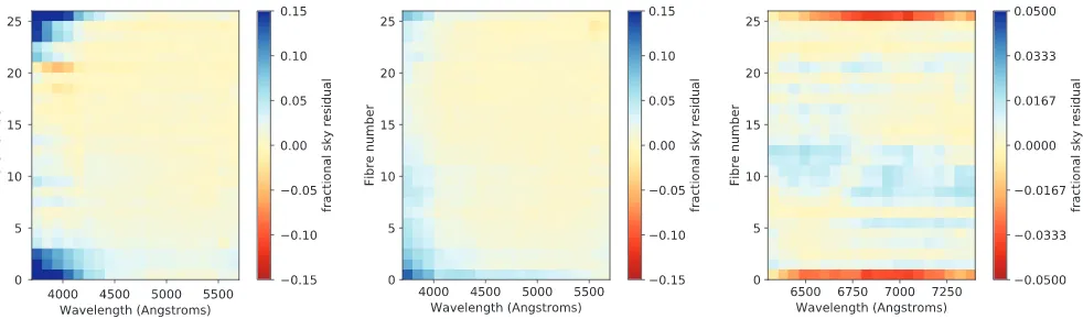
The improvements to profile measurement and fibre flat-fielding outlined in Section 2.2.1 lead to a substantial reduction in system-atic sky subtraction residuals, particularly in the blue arm of the

spectrograph. In Fig.3we show the median fractional sky

subtrac-tion residuals across 1750 individual data frames (for exposures of at least 900s), in 20 wavelength bins for each sky fibre in each arm of the spectrograph. The sky fibres are uniformly distributed along the slit, so systematic variations with sky fibre number re-late to variations along the slit. There is no change in the red arm residuals between DR1 and DR2. The DR2 residuals in the blue

arm (Fig.3, centre) are significantly reduced compared to the same

measurement from DR1 (Fig. 3, left), particularly at the corners

of the CCD. This reduction is because the new approach to fibre flat–fielding reduces the impact of ghost features present at these locations in the AAOmega spectrograph. Previously these features

were at the level of up to ∼20 per cent, but are now reduced to

Figure 3. The median fractional residuals in sky subtraction for SAMI sky fibres. From left to right we show the old residuals from DR1 in the blue, the new residuals for DR2 in the blue, and the new residuals for DR2 in the red (unchanged from DR1). For each sky fibre the flux is summed within 20 uniform bins in wavelength before determining the fractional residual. The median residual within each bin is then calculated across all object frames within the survey. Various low-level systematic trends can be seen, including increased residuals for the sky fibres at the very edges of the slit.

∼5 per cent or less. Other weak systematic features remain,

includ-ing a gradient at the level of∼1 per cent from top to bottom of the

CCD, higher residuals for the slit end fibres (fibres 1 and 26) and an increase for all fibres at the blue end. This last feature is largely driven by reduced S/N at the blue end of the blue arm, rather than any actual systematic reduction in sky subtraction accuracy.

We perform a second test of DR2 data quality that examines our improved spectral extraction and sky subtraction (see Section 2.2.1).

As we saw in Fig.3, there is a significant improvement in sky

sub-traction below 4000 Å at the top and bottom of the detector. This most strongly influences IFUs number 1 and 13 that are located at either end of the spectrograph slit. To demonstrate the improvement,

we measure the D4000n(Balogh et al.1999) and HδA(Worthey &

Ottaviani1997) indices for all spaxels with median S/N>10 from

galaxies that are contained within both DR1 and DR2. For SAMI DR1 the data in IFUs 1 and 13 (at the ends of the slit) show a

sys-tematic offset to lower values of D4000n(red contours and points in

Fig.4a). In contrast, the same spaxels in SAMI DR2 are completely

consistent with the distribution in the other IFUs (Fig. 4b). We

note that in this test we have not corrected the indices for emission

lines, so a small number of spaxels lie at lower HδAvalues than

might otherwise be expected (e.g. red points at D4000n1 and

HδA −4).

3.1.3 Flux calibration

We compare the flux calibration of SAMI DR2 data to SDSSg–

band images. The same procedure as described for the DR1 sample

in Green et al. (2018) is also carried out on DR2. This procedure

compares fluxes in SDSSg–band images and SAMI cubes within

an 8 arcsec diameter aperture. The SAMI cubes are convolved with

the SDSSg–band filter curve and the SDSS images are convolved to

the median seeing of SAMI. Galaxies with integrated fluxes below

100μJy were not included, to avoid extra scatter from low S/N. The

median flux ratio (SAMI/SDSS) is 1.048±0.003 (where the error

is the uncertainty on the median, not the RMS scatter), consistent

with results from DR1. As can be seen in Fig.5, the distribution

of flux ratios is slightly narrower for DR2 (solid line) than DR1

(dotted line). 95 per cent of objects have a flux ratio within±0.15

of the median. Regarding the accuracy of relative flux calibration, this is unchanged compared to previous data releases. As noted in

Allen et al. (2015), we find a colour offset,(g− r), of 0.043

with a standard deviation of 0.040, with respect to the SDSS PSF magnitude derived colours of the SAMI secondary standard stars.

3.1.4 WCS accuracy

During cube construction, we register the galaxy centroid in each individual dither by fitting a two-dimensional Gaussian to the ob-served flux. The dithers are aligned using these centroids, and are then combined such that the galaxy centre is located at cube spaxel coordinates (25.5, 25.5). We then assign the catalogue right as-cension (RA) and declination (Dec.) of the galaxy to this spaxel coordinate and define the World Coordinate System (WCS) of the cube relative to this position. While accurate for the majority of galaxies, there remains some uncertainty in the WCS due to the centroiding process, and, in a limited number of cases, the pipeline can misidentify the galaxy centre resulting in a significant offset.

We verify the accuracy of the WCS of the data by visual

inspec-tion and matching tor–band images from the Kilo Degree Survey

(KiDS; de Jong et al.2017). In Fig.6we show the offset in RA

and Dec. between the centre of the collapsed SAMI cube and the centre of the galaxy in the KiDS image. We find the mean offset is

−0.016±0.020 arcsec in RA and−0.102±0.017 arcsec in Dec.

When we remove catastrophic failures (see below), the mean offset

changes to−0.027±0.009 in RA and−0.106±0.008 in Dec.,

resulting in a decreased rms scatter, however the small statistically significant offset remains.

For cubes where multiple galaxies or a foreground star is present in the hexabundle or the galaxy is highly structured, the simple two-dimensional Gaussian fit can misidentify the galaxy centre, resulting in a large positional offset between the cube centre and the true galaxy centre. After visual inspection of the cubes, we determined

that 50 galaxies suffered from significant offsets (>1 arcsec in radial

offset) due to these issues. For these galaxies, we shift the cube WCS to match that determined from the KiDS imaging.

3.1.5 Seeing distribution

Each observation has an associated PSF, characterized by the FWHM. For individual observations these are measured by fitting a Moffat profile to the flux distribution of the secondary standard star. The output data cubes also have a PSF that depends on the

(a) (b)

Figure 4. The distribution of SAMI spaxels with median blue arm S/N>10 in the D4000nversus HδAplane for (a) data in SAMI DR1, and (b) data in

SAMI DR2. Only spaxels from galaxies that are common to both DR1 and DR2 are shown. IFUs 2–12 (black dashed contours and points) and IFUs 1, 13 (red contours and points) are shown separately. The improved DR2 data reduction leads to consistent locations in the D4000nversus HδAfor all IFUs. Contours

are linearly spaced in point density.

Figure 5. The distribution of flux ratios between SAMI cubes and SDSS images in theg–band using 8 arcsec diameter circular apertures. We compare SAMI DR1 (red dashed lines) and DR2 (solid black lines), with the vertical dotted lines showing the median flux ratio for each sample. Each histogram is normalized to the number of objects in the sample.

PSFs of the input observations, as well as the accuracy of regis-tering these inputs to a common coordinate system. In the upper

panel of Fig.7we show the FWHM of the PSF of the cube of

the secondary standard star as a function of the mean FWHM of

the input observations. For mean input FWHM1.5 arcsec, the

input and output FWHM are linearly related, with the PSF of the

cube being∼0.2 arcsec broader than the mean input PSF. In good

seeing, the difference between the cube PSF and the input PSF is increased. This is caused by two effects; the additional broad-ening in the output PSF due to uncertainties in the centroids of each input frame and the effect of the optical fibres, whose finite size effectively imposes a minimum FWHM on the PSF, even if atmospheric seeing is ignored. Atmospheric broadening is still the most significant factor in determining the FWHM of the output PSF.

In the lower panel of Fig.7we show the distribution of FWHM

for all galaxies in DR2, determined from Moffat profile fits to the secondary standard star cubes observed simultaneously with the galaxies. The mean FWHM of the output cubes is 2.06 arcsec,

varying between 1.10 and 3.27 arcsec. 84 per cent of galaxies have FWHM better than 2.5 arcsec.

4 C O R E DATA

The data in SAMI DR2 is broadly divided into core data, produced directly from the SAMI data reduction pipeline, and value-added data products, derived from SAMI Galaxy Survey science analysis pipelines. Here we describe the core data, with the data products being described in Sections 5 and 6.

4.1 Cubes

The primary data produced by the SAMI Galaxy Survey are pairs of spectral data cubes for each observed galaxy, covering the blue and red parts of the optical wavelength range. Each data cube consists

of 2048 spectral slices, where each slice is a 50×50 square area of

spatial pixels (spaxels). The sampling of the spatial axes is 0.5

arc-sec. For the blue cube the spectral sampling is 1.050 Å pixel−1_with

a spectral FWHM of 2.66 Å, covering the wavelength range 3650

to 5800 Å. For the red cube the spectral sampling is 0.596 Å pixel−1

with a spectral FWHM of 1.59 Å, covering the wavelength range

6240–7460 Å. See Table 1for further details. In addition to the

measured fluxes, each cube contains the variance, weight map, and

compressed covariance; see Sharp et al. (2015) for details.

4.2 Binned cubes

To complement the default cubes, we provide a set of three pre-binned data cubes, that we refer to as ‘adaptive’, ‘annular’, and ‘sectors’.

(i) Adaptive: Bins are adaptively generated to contain a target S/N of 10, using the Voronoi binning code of Cappellari & Copin

(2003). The S/N is calculated from the flux and variance spectra of

each spaxel as the median across the entire blue wavelength range.

Spaxels with S/N>10 are not binned.

(ii) Annular: Bins are generated as a series of elliptical annuli, centred on the centre of the cube. The position angle, PA, and

ellipticity, ε, of the galaxy are determined using thefind galaxy

PYTHONroutine of Cappellari (2002) from the image generated by

Figure 6. Offset between the SAMI cube WCS and KiDSr–band imaging. The left-hand panel shows the offsets for all DR2 galaxies. Note that 24 galaxies with large offsets lie outside the figure. The centre and right-hand panel show histograms of the offset in RA and Dec., respectively. Catastrophic failures have not been removed.

summing the cube along its wavelength axis. The spaxels are then allocated to five linearly spaced elliptical annuli, each with the PA

andεof the whole galaxy.

(iii) Sectors: Bins are generated as a series of elliptical annuli, with each annulus further subdivided azimuthally into eight regions of equal area. The axes of the sectors are defined in reference to the PA of the galaxy. The annuli are generated as for the annular binning scheme.

For each binned cube, we first generate a bin mask from the blue cube using the criteria described above, then sum the spectra for each spaxel contributing to a given bin to generate the binned spec-trum. The bin masks generated from the blue cubes are applied to the red cubes as well to allow direct comparison. The output

binned data cubes consist of 50×50×2048 arrays, maintaining

consistency with the original cubes. Each spaxel in the output cube contains the binned spectrum for the bin that it belongs to – spaxels from the same bin contain identical spectra. All spaxels containing flux are allocated to a bin. This procedure is repeated for the vari-ance cube, accounting for the covarivari-ance between spaxels in each

bin. We note that the variance of large bins (25 spaxels) may be

underestimated by up to 5 per cent due to a small component of unaccounted-for covariance between included spaxels (this will be corrected in future releases). Each binned cube consists of the flux and variance cubes and an additional bin mask image, indicating which spaxels have been combined into each bin. All binned data

are generated using thebinningmodule of the SAMI data

reduc-tion pipeline. Variareduc-tions on the adaptive and annular/sectors binning schemes can easily be generated by modifying functions within this module.

4.3 Aperture spectra

To facilitate comparison to existing single aperture surveys, we also provide a set of aperture spectra derived from the SAMI cubes.

These aperture spectra are generated using thebinningmodule of

the SAMI data-reduction pipeline as single-bin binned spectra, with two exceptions: spaxels lying outside the aperture are not allocated to a bin, and the flux of the aperture spectrum is re-scaled to ac-count for the difference in area between the included spaxels and the true bin area. The data format is also different; for each aperture we generate a one-dimensional flux array, a one-dimensional

vari-ance array (accounting for spatial covarivari-ance between contributing spaxels), and a two-dimensional bin mask image, indicating which spaxels have been summed to form the aperture. As for the binned data cubes, large apertures may have their variance underestimated

by up to∼5 per cent.

We provide six apertures, four of which are circular apertures

centred on the centre of the cube with diameter 1.4, 2, 3, and 4

respectively. We provide a fifth circular aperture with fixed physical diameter of 3 kpc, determined using the observed redshift of the galaxy from the GAMA survey and our adopted cosmology. The

sixth aperture is an elliptical aperture of major axis radiusRe, where

ε, PA, andReare taken from v09 of the GAMA S´ersic catalogue

(Kelvin et al.2012).

4.3.1 S/N

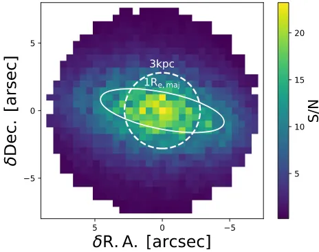
We estimate the aperture S/N by taking the median S/N value per Å between 4600 and 4800 Å in the rest frame. This range is clear of skylines and is fully contained within the SAMI blue arm. In

Fig.8we show histograms of the median S/N for the six available

apertures. We also show the median S/N map for a typical galaxy in

Fig.9, outlining theReand 3kpc apertures for reference. The 1Re

aperture spectra have a median S/N of 32; 92 per cent have an S/N above 10, and 25 per cent have a value above 50. The median S/N of the central pixel in the data cubes is 14 with a standard deviation of 13.

5 VA L U E - A D D E D DATA P R O D U C T S : E M I S S I O N - L I N E P H Y S I C S

For each of the core data products listed above (cubes, binned cubes, and aperture spectra), we fit strong emission lines arising from ionized gas and extract line fluxes, velocities, and velocity dispersions. From these we then create maps of value-added prod-ucts such as extinction maps (derived from the Balmer decrement), star-formation rate surface densities, and excitation mechanism classifications. We summarize here the emission line analysis, but note that the methods and products are very similar to those released

in DR1. We refer the reader to Green et al. (2018), Ho et al. (2016b),

and Medling et al. (2018) for further details on the emission-line

fitting and resulting data products.

Figure 7. Upper panel: comparison of the mean measured FWHM of in-dividual dithered exposures to the FWHM of the reconstructed secondary standard star cubes. FWHMs are from Moffat-profile fits. The dashed black line is the 1:1 relation. Lower panel: distribution of the FWHM in the re-constructed cube for all SAMI DR2 galaxies. The mean of the FWHM is 2.06 arcsec, and the standard deviation is 0.40 arcsec.

5.1 Emission-line fitting

We fit seven strong optical emission lines within the SAMI

wavelength range: [OII]3726+3729, Hβ, [OIII]5007, [OI]6300,

Hα, [NII]6583, [SII]6716, and [SII]6731. We also fit the lines

[OIII]4959 and [NII]6548, but their fluxes are fixed to their

phys-ical ratios relative to the stronger [OIII] and [NII] lines. Using

version 1.1 of theLZIFU software package (Ho et al.2016a), we

stitch together the blue and red spectra accounting for the differing spectral resolution (Section 3.1.1). We then subtract the underly-ing stellar continuum before fittunderly-ing each emission line with one to three Gaussian profiles. The Gaussian profiles are fit using the

Figure 8. Histograms of the aperture S/N for all DR2 galaxies, in the six available apertures. The S/N is the median value in the range from 4600 to 4800 Å. The median value in each aperture is included in the line labels.

Figure 9. The median S/N per Å in the blue cube for GAMA ID 91926. The median is measured between 4600 and 4800 Å. The white lines show the relative sizes and shapes of two of the six available apertures; the solid line outlines the elliptical aperture with 1Resemi-major axis, and the dashed

line shows the circular aperture of 3 kpc diameter. For this galaxy, the S/N per Å in both the 3 kpc diameter andResemi-major aperture spectra are 51.

Levenberg–Marquardt least-square method implemented in (MPFIT;

Markwardt2009). All selected emission lines are then fit

simulta-neously with each kinematic component constrained to the same velocity and velocity dispersion. From the Gaussian fits, we obtain the emission line fluxes, velocities, and velocity dispersions.

For the spectral cubes (Section 4.1), we follow DR1 in providing both a 1-component Gaussian fit capturing the bulk emission and gas motions, and a multicomponent fit. The multicomponent fit cap-tures both the dominant gas emission and fainter velocity struccap-tures such as outflows, and represents a more accurate total gas emission.

Each spaxel is fit 3 times using LZIFUto obtain one-, two-, and

three-component fits to each emission line. The number of compo-nents in the multicomponent fits are determined using an artificial neural network trained by astronomers (for full details on the neural network, and precision success with SAMI data, see Hampton et al.

2017).

One significant difference between the emission line fits to the spectral cubes provided in DR2 relative to DR1 is the fitting of the underlying stellar continuum. In DR1, the stellar continuum was fit on a spaxel-by-spaxel basis using the penalized pixel-fitting routine

(PPXF; Cappellari & Emsellem2004; Cappellari2017), even when

the S/N in the continuum was low. Doing so can lead to large uncertainties in the correction for the underlying absorption lines, specifically impacting the Balmer emission lines. To account for this impact, we included an additional systematic uncertainty in the

Balmer lines (described in Medling et al.2018).

In DR2, we now use the significantly improved stellar contin-uum fitting to better subtract the contincontin-uum prior to fitting the emission lines. Here, we give a brief description of the contin-uum fitting procedure and refer to Owers et al. (in preparation) for further details. We use the Voronoi-binned data, which has

S/N∼10 in the continuum, to constrain the number of templates

that are used to fit each spaxel within the Voronoi bin of interest.

This is achieved by usingPPXF to fit the Voronoi-binned

spec-trum with a subset of the MILES simple stellar population (SSP)

spectral library (Vazdekis et al.2010) that contains four

metallic-ities ([M/H] = −0.71,−0.40, 0.00, 0.22) and 13 logarithmically

spaced ages ranging from 0.0063 to 15.85 Gyrs. Following Cid

Fernandes et al. (2013), the MILES SSPs are supplemented with

younger SSP templates drawn from Gonz´alez Delgado et al. (2005)

with metallicities [M/H] = −0.71,−0.40, 0.00, and ages 0.001–

0.025 Gyr. During the fitting, emission line templates are included for the Balmer lines, as well as strong forbidden lines. Importantly, this simultaneous fitting of emission and absorption components allows the regions surrounding the age-sensitive Balmer lines to be included in the continuum fits. The stellar kinematics are not fitted for during this process, and are fixed to the values determined in Section 6.1.

The subset of SSP templates that have non-zero weights assigned in the fits to the Voronoi binned spectra is then used during the fitting of each spaxel contained within the region defined by the Vorenoi bin. Again, emission lines are fitted simultaneously, and the stellar kinematics are fixed to those determined in Section 6.1,

while allowingPPXF to re-determine the optimal template weights

only for spaxels where the S/N>5. For spaxels with S/N<5, the

weights determined during the Voronoi binned fitting are used to produce a single optimal template, while the stellar kinematics are fixed to those derived from the Voronoi-binned data. This helps to

guard against poor fits due to low S/N. In all of thePPXF fitting

described above, we include a 12th-order multiplicative polynomial.

This continuum fit is then used inLZIFUto subtract the continuum

and measure the final line fluxes for the 1- to 3-component fits. Overall this method produces similar line fluxes to those found in DR1, but with better constraints in spaxels with low-S/N continua, and some systematic offsets in galaxies with significant Balmer absorption features.

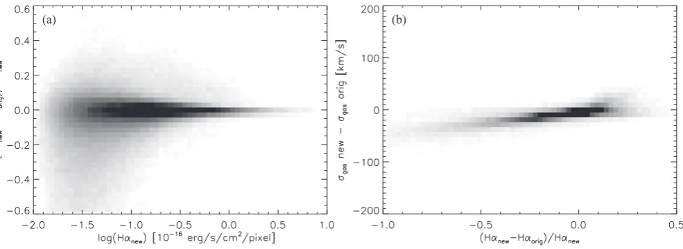
In terms of the Hαemission line flux, for most pixels with low

continuum S/N the new continuum fitting procedure produces a

similar line flux, especially for strong lines. Fig.10a shows a 2D

density diagram of the relative difference in 1-component Hαflux

for the original DR1 and new DR2 continuum fitting methods for

all spaxels with significant line emission (HαS/N>5) and weak

continuum (S/Ncont<10). The median relative difference for all

spaxels is 0.003, but with a standard deviation of 0.3, with these differences clearly increasing for low line fluxes. The majority of

spaxels (∼80 per cent) have Hαfluxes that agree within 10 per cent,

and only∼6 per cent of the low continuum S/N spaxels disagree by

more than 30 per cent.

To reveal the origin of this change, we show the relative

differ-ence of Hαflux against the difference in determined gas velocity

dispersion in Fig.10b. We again show this for all spaxels with

sig-nificant line emission (HαS/N>5) and weak continuum (S/Ncont<

10). All spaxels with similar Hαfluxes show similar velocity

dis-persions, but for spaxels with a substantially different Hαflux we

see that the velocity dispersion of the original method is also sys-temically different, arising from an improperly determined Balmer absorption feature in the low continuum S/N.

With the aim of understanding the systematic effects of the differ-ent continuum fitting procedures between DR1 and DR2, we inves-tigate whether the Balmer decrements measured using higher-order Balmer emission lines depart from the expectations of a Calzetti dust extinction law. These tests are similar to those performed by

Groves, Brinchmann & Walcher (2012) for the SDSS. To do this,

we select a subset of the DR2 galaxies that have more than 10

high-quality (continuum S/N>5) spaxels that are classified as

star-forming, and have well-detected Hβand Hαfluxes (S/N>5). For

the high-quality star-forming spaxels in these galaxies, we measure

emission fluxes for the Balmer lines Hε, Hδ, Hγ, and Hβusing

direct summation in windows surrounding those lines. The window

width is set to±3σwinaround the redshifted line centre, whereσwin

is defined by the quadrature sum of the instrumental resolution and

the gas-velocity dispersion determined by the 1-componentLZIFU

fits. The redshift used to determine the line centre includes

contribu-tions from both the galaxy redshift and the gas velocity fromLZIFU.

For each line, we measure two sets of emission line fluxes: one af-ter subtracting the continuum defined using the procedure outlined for DR1, and another after subtracting the continuum measured as outlined above. The emission line fluxes are corrected for Galactic extinction, and then used to measure Balmer decrements for the higher order lines.

In Fig.11for each galaxy we plot the median value of the higher

order Balmer decrements against the median Hα/Hβdecrements,

where Hαand Hβare determined from theLZIFUfits, and are also

corrected for Galactic extinction. The decrements are normalized by the theoretical value for Case B recombination. The red line

shows the expected trend due to a Calzetti et al. (2000) extinction

law. In the top panels, the results derived using the new continuum fitting are shown, while the bottom panels show the results from the DR1 continuum fitting method. Neither the new continuum fitting method used for DR2, nor the method used in DR1 produces results

that align with the expectations of a Calzetti et al. (2000) extinction

law. However, the DR2 results show both a smaller offset and scatter when compared with the DR1 results, and this is particularly true for

the Hδ/Hβand Hε/Hβratios shown in the middle and right-most

panels, respectively.

Given that we have selected only relatively high S/N spaxels, the difference in the results from the two continuum fitting methods is likely driven by two changes. First, in DR2 we now modulate the SSP templates with a multiplicative polynomial rather than the additive polynomial used in DR1. Second, we now simultaneously fit for emission and absorption in the vicinity of the Balmer lines, whereas previously these regions were masked during the fit. The combined effect of using an additive polynomial alongside masking the age-sensitive Balmer lines was that younger templates were often excluded from the fit; the blue flux was modelled by the additive polynomial rather than a young stellar population, thereby underestimating the Balmer absorption at bluer wavelengths. We

note that the offset observed in the new DR2 values in Fig.11is

similar to that noted by Groves et al. (2012) for SDSS DR7 data.

Investigation into the origin of the offset is ongoing. At this stage

(a) (b)

Figure 10. Comparison of the LZIFU determined 1-component Hαflux based on the original DR1 continuum method and the new DR2 continuum method. All spaxels with weak continuum (S/Ncont<10) and significant line detection (S/NHα>5) in DR2 are examined here. (a) A 2D density histogram of the relative difference in Hαflux as a function of the new DR2 continuum Hαflux. (b) A 2D density histogram showing how the relative difference in Hαflux between the two methods correlates with the difference in the determined gas velocity dispersion between the two methods. These figures demonstrate that the majority of spaxels are consistent (>80 per cent), but at weak line flux (<2.10−17erg/s/cm2/pixel), errors in the Balmer line absorption feature due to poor continuum fitting in the original DR1 method lead to weak but incorrect broad lines.

this alternative continuum fitting approach has been applied to the original spectral cubes only because they are more susceptible to inaccurate continuum subtraction due to their typically lower S/N than the other spectral data products.

In addition to the original spectral cubes, we also provide emis-sion line fits for the binned cubes (Section 4.2) and aperture spectra (Section 4.3). For the adaptively binned and sectors-binned spectral cubes, we follow the same conventions as for the original spectral cubes, providing both 1- and multicomponent fits.

For the annular-binned spectral cubes we provide only

2-component fits, and fit the stellar continuum directly withinLZIFU

usingPPXF given the higher continuum S/N. Only 2-component fits

are provided given that in many cases rotation dominates the emis-sion structure in the outer bins leading to double-horned profiles that require two separate components to be fit.

All aperture spectra are also fit usingLZIFU, treating each

spec-trum as an individual spaxel. As with the original cubes we pro-vide both 1-component and multicomponent fits to the aperture spectra. These are provided as tabulated line fluxes, gas velocities (relative to the input heliocentric GAMA redshifts) and velocity dispersions, and associated errors for all apertures described in Section 4.3.

5.2 Star formation rates and other products

As in DR1, we also release higher-order data products based upon the emission line fitting: Balmer decrement-based attenuation maps, classification of star-forming regions, and star formation rates. For full details on the determination of these products, we refer the

reader to Medling et al. (2018), but briefly summarize these here.

We present the attenuation maps as correction factors,FHα for

the Hαemission line. Using the Balmer decrement (Hα/Hβ) and

assuming a Cardelli, Clayton & Mathis (1989) extinction law, we

determine this as

Fattenuate=

1

2.86

Hα

Hβ

2.36

, (1)

where Hα/Hβintr =2.86 is the intrinsic flux ratio of the Balmer

decrement (assuming Case B recombination, Te = 104K and

ne=100 cm−3). For regions where the Hβ line is not detected

or Hα/Hβ < 2.86, we setFattenuate = 1 and the associated

er-rorδFattenuate = 0. Note that the Hβ non-detection regions may

also be high attenuation regions, so this correction factor repre-sents a lower limit in these cases. Also note that for the original resolution and adaptively binned data, the Balmer lines need to be

smoothed by a Gaussian kernel of FWHM=1.6 spaxels (0.8

arc-sec) to account for the different PSFs before the determination of the Balmer decrement and attenuation correction maps as described in

Medling et al. (2018), because of the issue of aliasing arising from

differential atmospheric refraction (described in detail in Green

et al.2018).

For all spaxels we also classify whether the emission-line spec-trum is dominated by photoionization by massive stars associated with recent star formation, or by other mechanisms (such as active galactic nucleus, shocks, etc.). This is done using cuts on emission line ratio based upon the classification scheme described in

Kew-ley et al. (2006) and fully described in Medling et al. (2018). For

both the original and binned data we present these as star formation masks, where any spaxel dominated by mechanisms other than star formation are set to 0.

We present star formation rate maps for both original and all binned cubes by first creating attenuation-corrected, star

formation-dominated Hαmaps. We then convert this to a star formation rate,

using the Kennicutt, Tamblyn & Congdon (1994) calibration

con-verted to a Chabrier (2003) stellar IMF:

SFR [Myr−1]=5.16×10−42FHα[erg s−1]. (2)

Note that, due to both the removal of contaminated regions via the star formation masks and missing heavily obscured regions

where Hβand even possibly Hαare undetected, these maps likely

represent lower limits to the true current star formation in the galaxies.

Figure 11. Comparison of the higher-order Balmer decrements derived from emission line fluxes measured after subtracting continua using the continuum fitting method used in DR2 (top row) and the continuum method used in DR1 (bottom row). The comparisons are made for Hγ/Hβ, Hδ/Hβ, and Hε/Hβ, determined by direct summation over a narrow window around the line centre (left-hand, middle, and right-hand panels), with the Hβ/Hαratio shown on the x-axis, taken from the LZIFU fits. The red line shows the trend in the Balmer decrements of interest derived from a Calzetti et al. (2000) extinction law. We see an improvement in both the magnitude of the offset and the scatter in the distribution when comparing DR2 with DR1, although the offsets from the Calzetti et al. (2000) line are in the opposite sense.

6 VA L U E - A D D E D DATA P R O D U C T S : A B S O R P T I O N - L I N E P H Y S I C S

6.1 Stellar kinematics

6.1.1 Method

Stellar kinematic parameters are extracted from the SAMI cubed data following the method described in detail in van de Sande et al. (2017b). We use thePPXF code to fit all spectra. Our method is summarized below.

SAMI blue and red spectra are combined by first convolving the red spectra to match the instrumental resolution in the blue. We

use the codeLOG REBINprovided with thePPXF package to rebin

the combined blue and red spectra on to a logarithmic wavelength

scale with constant velocity spacing (57.9 km s−1_{). We use annular}

binned spectra (Section 4.2) to derive local optimal templates from

the MILES stellar library (S´anchez-Bl´azquez et al.2006) that

con-sists of 985 stars spanning a large range in stellar atmospheric pa-rameters. A Gaussian line-of-sight velocity distribution (LOSVD)

is assumed, i.e. we extract only the stellar velocityV and stellar

velocity dispersionσ.

After the optimal template is constructed for each annular bin, we

runPPXF three times on each galaxy spaxel. For every step, we mask

the following emission lines: [OII], Hδ, Hγ, Hβ, [OIII], [OI], Hα,

[NII], and [SII], even if no emission lines are detected. The first fit

is used for determining a precise measure of the noise scaling from the residual of the fit. We use an additive Legendre polynomial to remove residuals from small errors in the flux calibration, and as

in van de Sande et al. (2017b), we demonstrated that a 12th-order

additive Legendre polynomial is sufficient for SAMI data. In the

second fit, we clip outliers using the CLEAN parameter inPPXF.

In the third and final iteration,PPXF is allowed to use the optimal

templates from the annular bin in which the spaxel is located, as well as the optimal templates from neighbouring annular bins.

Uncertainties on the LOSVD parameters are estimated using a Monte Carlo approach. We estimate the uncertainties on the LOSVD parameters for each spaxel from the residuals of the best fit minus the observed spectrum. These residuals are then randomly

ranged in wavelength and added to the best-fitting template. This

simulated spectrum is refitted withPPXF, and we repeat the

pro-cess 150 times. The uncertainties on the LOSVD parameters are the standard deviations of the resulting simulated distributions.

We follow the same method for the binned data (Section 4.2). For the aperture spectra (Section 4.3), we construct an optimal template for each individual aperture and then use the same procedure as described above to extract the LOSVD.

We note that the varying spectral resolution from fibre to fibre (Section 3.1.1) can have a significant impact on the stellar kinematic measurements if the intrinsic stellar dispersion is close to or less

than the instrumental dispersion (Federrath et al.2017; Zhou et al.

2017). However, the stellar kinematic measurements are obtained

from the cubed frames, where a dither pattern is applied. As individ-ual spaxels are constructed from a combination of multiple fibres, the spectral resolution will be an average of all the contributing fibres. We do not consider the changing resolution as a function of wavelength to be significant enough to impact the extracted stellar kinematic measurements, as those are derived from a simultane-ous fit over the entire wavelength range, and the full wavelength variation is comparable to the fibre-to-fibre variation.

6.1.2 S/N estimate from the stellar kinematic fits

Residuals from the observed spectrum minus the best-fitting tem-plate provide a good test of the accuracy of the variance spectra. Here, we compare the S/N derived from the flux and variance spec-trum to the S/N derived from the stellar kinematic best-fit residual for every unbinned spaxel that meets the quality criteria in the next Section 6.1.3. The variance spectrum S/N was derived in the blue wavelength region between spectral pixel 1100 and 1600 (approx-imately between 4500 Å and 5000 Å), whereas the S/N from the

residuals is determined for all ‘goodpixels’ in thePPXF fit (i.e.

ex-cluding emission lines and 3σ outliers). Therefore, we stress that

this comparison should be considered a consistency check, not an exact derivation of the cube variance scaling.

In the left-hand panel of Fig.12 we find that>95 per cent of

the data are above the one-to-one relation, which indicates that the variances may be slightly overestimated. While there are

consider-ably fewer data-points aboveS/N50, the scatter between the two

S/N estimates becomes increasingly larger and the S/N from the best-fitting residual drops below the S/N from the variance spec-trum. However, we note that at this high S/N, uncertainties from the adopted stellar library, template mismatch, and other fitting related issue are starting to dominate the residual S/N estimate.

Thus, above S/N ∼ 50, the S/N comparison becomes harder to

interpret.

We show the distribution of both S/N estimates in the

right-hand panel of Fig.12. Note that we only show data where the S/N

estimated from the variance spectrum is greater than 3 Å−1_{, as lower}

S/N spaxels are not fit by the stellar kinematics pipeline. As before, we find that the median variance spectrum S/N is lower than the S/N derived from the best-fitting residual. The difference in medians is 16.6 per cent. Thus, while we find that the DR2 variances may be slightly overestimated, we conclude that this offset is relatively mild.

6.1.3 Kinematic quality cuts

For SAMI data we recommend applying the following quality

cri-teria to the stellar kinematic data: signal-to-noise (S/N)>3 Å−1_,

σobs>FWHMinstr/2∼35 km s ,Verror<30 km s (Q1from van

de Sande et al.2017b), andσerror< σobs∗0.1 + 25 km s−1(Q2from

van de Sande et al.2017b).

For kinematic data products such asKINEMETRY, the kinematic

PA,V/σ, andλR, we have additional flags. We perform a visual

in-spection of all 1559 SAMI kinematic maps and exclude 42 galaxies with irregular kinematic maps due to nearby objects or mergers that influence the stellar kinematics of the main object. We furthermore

exclude 481 galaxies whereRe<1.5 or where eitherReor the radius

out to which we can accurately measure the stellar kinematics is less

than the half-width at half-maximum of the PSF (HWHMPSF). This

brings the final number of galaxies for which we can derive reliable 2D stellar kinematic data products to 1036. The number of galaxies

withReaperture velocity dispersion measurements is 1171.

6.1.4 Aperture velocity dispersion comparison

We compare our aperture velocity dispersion values to measure-ments from SDSS 3-arcsec single-fibre spectra. We refit the SDSS spectra, using the same technique and templates as described in Section 6.1.1. Our values are in good agreement with the stan-dard SDSS pipeline velocity dispersions and the measurements by

Thomas, Maraston & Johansson (2011). We show the comparison in

Fig.13, where any measurements with (S/N)SDSS<5 Å−1,σobs<

FWHMinstr/2, and σerror> σobs∗0.025 + 10 km s−1are excluded.

The first and last quality criteria are stricter than described in Sec-tion 6.1.3 due to the higher mean S/N of the SAMI and SDSS

aper-ture spectra. We quantify the comparison, using the medianσoffset

(σSDSS−σSAMI) and the fractional dispersion difference,σ =

(σSDSS−σSAMI)/σSAMI. There is excellent agreement between the

SAMI and SDSS measurements when the velocity dispersion is

higher than the SAMI instrumental resolution of∼70 km s−1

(me-dianσ offset =1.4 km s−1_{, RMSσ =0.10), or when the S/N}

of the SAMI aperture spectra is greater than 25 per Å (medianσ

offset =1.9 km s−1_{, RMSσ =0.12). Below 70 km s}−1_{, we find}

a larger medianσ offset =14.9 km s−1_{and the RMS scatter in}

σincreases to 0.47, but we note that the majority of galaxies with

low-velocity dispersion also have the lowest S/N.

Below the instrumental resolution we detect a deviation from the one-to-one relation; the SDSS velocity dispersions are increasingly higher than the SAMI measurements. This hints at a systematic bias

in the SDSS velocity dispersions at lowσ. Note that it is extremely

difficult to reconstruct an exact SDSS single-fibre measurement using IFS data; the SDSS aperture is circular, convolved with an observed PSF, and differential atmospheric refraction cannot be corrected for. Thus, we believe the SAMI aperture spectra to be more reliable for three reasons. First, the SDSS spectrograph is mounted on the telescope near the Cassegrain focus and therefore suffers from flexure that can change the spectral resolution, whereas the SAMI-AAOmega is a bench-mounted spectrograph and is therefore more stable. Secondly, the S/N in the SAMI spectra is higher, and thirdly

our simulations of the recovery ofσfrom synthetic SAMI spectra

do not reveal a systematic offset below the instrumental resolution

(Fogarty et al.2015) in the SAMI measurements.

There are two notable outliers at the highest SAMI veloc-ity dispersion, where the SDSS velocveloc-ity dispersion is

signifi-cantly lower than the SAMI value (σSDSS∼250 km s−1 versus

σSAMI∼300 km s−1, respectively). A closer investigation of these

two objects revealed that one galaxy is a merger remnant with strong emission lines, where a small misplacement of the fibre centre can cause a large change in the velocity dispersion. The second object