An Efficient Bayesian Approach to Multiple Structural Change in Multivariate Time Series

Munich Personal RePEc Archive

An Efficient Bayesian Approach to

Multiple Structural Change in

Multivariate Time Series

Maheu, John M and Song, Yong

McMaster University, University of Melbourne

May 2017

Online at

https://mpra.ub.uni-muenchen.de/79211/

An Efficient Bayesian Approach to Multiple Structural

Change in Multivariate Time Series

∗

John M. Maheu

Yong Song

First draft Dec 2015

This draft May 2017

Abstract

This paper provides a feasible approach to estimation and forecasting of multi-ple structural breaks for vector autoregressions and other multivariate models. Due to conjugate prior assumptions we obtain a very efficient sampler for the regime al-location variable. A new hierarchical prior is introduced to allow for learning over different structural breaks. The model is extended to independent breaks in regres-sion coefficients and the volatility parameters. Two empirical applications show the improvements the model has over benchmarks. In a macro application with 7 variables we empirically demonstrate the benefits from moving from a multivariate structural break model to a set of univariate structural break models to account for heterogeneous break patterns across data series.

∗_{Maheu thanks SSHRC of Canada for financial support and the 2015 Eminent Research Scholarship,}

University of Melbourne.

†_{DeGroote School of Business, McMaster University and RCEA. Email:[email protected]}

1

Introduction

Multivariate time series data plays a central role in macroeconomic analysis and prediction. Linear models such as vector auto regressions (VAR) are standard tools to calculate the impulse response function and forecasts. Recently, many papers have highlighted the impor-tance of nonlinearity associated with structural instability for macroeconomic and financial variables such as GDP growth, real interest rate, inflation and equity returns among many others. However, because the estimation usually involves intensive computation, most of the point models are applied to univariate time series. Existing multivariate change-point models have restrictions on the number of regimes a priori. It is either fixed at a small number (2 or 3) as in Jochmann and Koop (2011) or assumed equal to the length of the data as in Cogley and Sargent (2005). A multivariate approach which can estimate and forecast in the presence of an unknown number of regimes is missing in the current literature. This paper develops a new multivariate time series model to fill the gap by exploring the full posterior distribution for the allocation of the data to their respective regimes. The speed of estimation of the new approach is increased by using a conjugate prior for the parameters which characterize each regime. The simulation of the regime allocation of the data from its posterior distribution is very efficient, because the time-varying parameters for the condi-tional data density are integrated out. A new hierarchical structure is introduced to exploit the information across regimes.

Accounting for structural instability in macroeconomic and financial time series modeling and forecasting is important. Empirical applications by Clark and McCracken (2010), Gior-dani et al. (2007), Liu and Maheu (2008), Wang and Zivot (2000) and Stock and Watson (1996) among others demonstrate strong evidence for the existence of nonlinearity in the form of structural changes.

The challenges of estimation and forecasting in the presence of structural breaks has been recently addressed by Koop and Potter (2007), Maheu and Gordon (2008) and Pesaran et al. (2006) by using Bayesian methods. These approaches provide feasible solutions for univariate time series modeling, but they are computationally intensive. This is because there are so many combinations of break points that exploring them exhaustively is impractical.1 Extending these methodologies to the multivariate framework is empirically unrealistic, since a multivariate model requires much more computation as the number of variables increases. Instead this paper extends the efficient posterior sampling methods for univariate structural break models in Maheu and Song (2014) to the multivariate setting.

Current multivariate change-point models include Cogley and Sargent (2005), Jochmann and Koop (2011), Koop et al. (2011) and Pettenuzzo and Timmermann (2011). A common feature of these models is that they need to fix the number of regimes a priori. The full posterior distribution for the allocation of the data to their respective regimes is not ex-plored because of this restriction. One potential solution to this problem is to estimate the

1

For example, Koop and Potter’s (2007) model assumes path dependent time-varying parameters, which imply O(2T

) possible change-points scenarios. Although they have reduced the state space from O(2T

) to

O(T2

) in their MCMC algorithm, it is still computationally challenging to calculate the predictive density and the mixing property of their MCMC algorithm is left unanswered. Another approach with an unknown number of regimes is Maheu and Gordon (2008). Since their approach requires conductingO(T2

model many times. For each time, the estimation is associated with a distinct number of regimes. However, this solution is computationally expensive and in each single estimation a multimodal posterior density may exist, which can cause slow mixing of the Markov chain and affect the inference.

To alleviate the computational burden, we use a conjugate prior for the parameters which characterize each regime. This assumption avoids the numeric approximation of the conditional posterior distribution and provides a closed-form predictive density. This results in a large gain in computational speed. Meanwhile, another advantage of this methodology is that the sampler of the regime allocation is very efficient since the parameters which characterize each regime can be integrated out as nuisance parameters.2

Some may regard the conjugate prior as a drawback of our approach. This assumption is necessary to achieve the closed form results and computational benefits. Conjugate priors to VAR was investigated by Kadiyala and Karlsson (1997) for the practitioners. Recent empir-ical work such as Carriero et al. (2015) has shown the usefulness of simple conjugate priors for the U.S. economy. Banbura et al. (2010) augment the conjugate prior with a shrinkage parameter to reflect subjective belief and show that it is competitive in forecasting. These methods are applied to linear models without structural change. They have demonstrated that a conjugate prior is practically reasonable and a good prior for our structural change models.

Regarding prior elicitation for the parameters which characterize each regime, we adopt two different but closely related approaches. The first is a slightly revised simple conjugate prior used in Carriero et al. (2015), which is designed to approximate the Minnesota prior (Litterman 1986). This prior is informative but covers a reasonable range of the parameter space. The advantage of this prior is the fast computational speed. For instance, if we assume a VAR(1) model in each regime in a 7-variable system for 600 observations, it takes less than 5 seconds to simulate 6000 samples of model parameters from the posterior distribution on a regular desktop PC.3

The second new prior features a hierarchical structure with shrinkage hyper parameters. The hierarchical structure is on the parameters which characterize each regime. It is designed to exploit the information across regimes (Pesaran et al. 2006). In addition, the shrinkage method (e.g., Belmonte et al. (2014)) makes the model parsimonious in the Bayesian frame-work. The shrinkage hyper parameters in our model can shrink the second prior towards the first one. It reflects the prior belief for the variation of the hierarchical structure.

The hierarchical structure in this paper, to the best of our knowledge, is new to the mul-tivariate time series literature. Current literature of the hierarchical priors such as Pesaran et al. (2006) or Koop and Potter (2007) are for a univariate setting. In our new approach, besides the ability to learn across regimes, the hierarchical prior is systematically calibrated by following the first prior, which approximates the Minnesota prior. This feature is very important for multivariate models because of the overparameterization problem. In other words, the curse of dimensionality may make a seemingly harmless hierarchical prior have a strong impact on the inference. Since our hierarchical prior is built on the Minnesota prior, it has a solid theoretic foundation and a reasonable range for the model parameters.

2

This is called Rao-Blackwellisation. See Casella and Robert (1996).

3

In order to apply the joint sampler for the time-varying parameters, assuming path in-dependence is necessary to reduce the dimension of the state space. This paper applies the assumption similar to Chib (1998) to reduce the dimension of the state space from O(2T₎

to O(T). Specifically, we assume that the data before a break point is uninformative for the current regime conditional on the prior for the parameters characterizing each regime. For the non-hierarchical model, this assumption is equivalent to Chib (1998). For the hi-erarchical approach, the parameters which characterize each regime are dependent, because they share the same hierarchical prior and this prior is not exogenously fixed. However, they are independent conditional on one sample of the hierarchical prior parameters. This assumption frees the model from path dependence and enables an exhaustive exploration of the posterior for the regime allocation. By using this assumption, we have maximal T

paths for each observation, which can be evaluated very quickly after being combined with the conjugate prior assumption.

In summary, our approach has five attractive features for practitioners. First, the number of regimes is estimated endogenously and the regime allocation is explored from its posterior distribution exhaustively. All time-varying parameters are sampled jointly, so the estima-tion is efficient in terms of mixing. Second, the conjugate prior makes the estimaestima-tion of the non-hierarchical model very fast because no numeric approximation is involved. Third, the hierarchical structure with shrinkage control is parsimonious and able to exploit the information across regimes to improve forecasting. Multiperiod out-of-sample forecasts in-corporate the probability of multiple structural breaks out-of-sample. Lastly, the priors are automatically adjusted to different normalizations, because they are calibrated according to the Minnesota prior.

Besides the need for a conjugate prior, a second potential issue is that all parameters en-tering the data density are assumed to break simultaneously.4 _{We extend the model to allow} for independent breaks in regression parameters and covariance parameters5_{, nevertheless, if} all or a subset of parameters are breaking independently a time-varying parameter models may perform better as we show in one application.

Two empirical applications are considered. The first is an application to oil and real GDP. The multivariate hierarchical structural break models produce superior density forecasts for several forecast horizons compared to a number of popular benchmark specification. Several break points are identified and in general, the hierarchical prior is significantly better in terms of Bayes factors compared to the structural break model without this prior specification. In the second application to a macro model with 7 variables we find the univariate hierarchical structural break model of Maheu and Song (2014) applied to each data series independently produces the best density forecasts. Point forecasts from the structural break models are competitive and are generally best from the univariate specifications. These results under-score the importance of allowing parameters to break at different times. Posterior estimates of break patterns in the different univariate models display considerable heterogeneity.

The paper is organized as follows. The next section introduces the benchmark multivari-ate linear model, conjugmultivari-ate prior and posterior. Section 3 details the multivarimultivari-ate structural

4

We thank a referee for pointing out the importance of this issue.

5

break model followed by Section 4 which extends the model with an hierarchical prior as well as independent break processes for the regression parameters and covariance matrix. Sec-tion 5 discusses out-of-sample forecasts that account for in-sample breaks as well as breaks out-of-sample. Two empirical applications to oil and real GDP and a 7 variable VAR are given in Section 6 and 7. Conclusions are found in Section 8 followed by the Appendix that collects additional details on posterior simulation.

2

Multivariate Linear Model

We start with a multivariate linear model for aN×1 vectoryt= (y1t, y2t, ..., yN t)′ as follows:

yt = Φ

′

xt+et, et

i.i.d.

∼ N(0,Σ), (1)

wherext is aM×1 vector of independent variables and Φ is aM×N matrix of coefficients.

Each et is a N ×1 iid normal random vector with zero mean and a covariance matrix Σ.

Let T represent the length of the time series data. Define Y = (y1, y2, . . . , yT)′, X =

(x1, x2, . . . , xT)′ and E = (e1, e2, . . . , eT)′. Then, we can write (1) as

Y =XΦ +E, E ∼M N(0,Σ, IT). (2)

The dataY isT×N,X isT×M and the error termE isT×N. The notationM N(0,Σ, I) means the matrix normal distribution. The first parameter is a T ×N zero matrix rep-resenting the mean of the error matrix E. The second parameter Σ is a N ×N matrix and equals to the covariance of et. The last parameter, IT, is a T ×T identity matrix and

proportional to the covariance matrix of each column of the matrix E. The identity matrix

IT comes from the assumption thatet is i.i.d. If vectorizing the matrixE, the matrix normal

distribution is equivalent to a multivariate normal distribution as vec(E) ∼ N(0,Σ⊗I) or vec(E′

)∼N(0, I⊗Σ).

This paper focuses on structural change in the VAR model. For a VAR(p) model, where

p is the number of lags in the autoregression, it can be represented as

yt =φ0+φ1yt−₁+...+φ_py_t−_p+e_t

and can be cast into the above model with xt = (1, yt′−₁, y ′

t−₂, . . . , y

′ t−_p)

′

, M = N p+ 1 and Φ = (φ0, φ1, . . . , φp)′.

2.1

Prior

We assume an Inverse Wishart-Matrix Normal prior distribution for (Φ,Σ) as Carriero et al. (2015):

Σ∼IW(S, ν), (3)

Φ|Σ∼M N(Φ,Σ,Ω). (4)

1. A stationary series has its regression coefficients centered around 0. A non-stationary series has its regression coefficients approximating the random walk.

2. The prior for a distant lag is tighter than for a closer lag. In other words, the coefficients of the regressors shrink to zero as their lag length increases.

3. The volatility and intercept are calibrated by using the univariate series information.

Define the variance of the error term from the best fit ARIMA model of yi as ˆvi2. The

priors are set as follows:

1. We set ν=N + 3.5, S_ii= (ν−N −1)ˆv2

i and Sij = 0 ifi6=j. So we have

E(Σ) =

     ˆ v2

1 0 ... 0 0 ˆv2

2 ... 0 ... ... ... ...

0 0 ... vˆ2

N      ,

with sd(Σii) = 2ˆvi2 and sd(Σij)≈1.2ˆvivˆj if i6=j.

2. We set

Φ =             

0 0 ... 0

1(nonstationary) 0 ... 0

0 1(nonstationary) ... 0

... ... ... ...

0 0 ... 1(nonstationary)

0 0 ... 0

... ... ... ...

0 0 ... 0

            

If a seriesyi is nonstationary, we set the corresponding coefficient to 1 and 0 otherwise.

Stationarity can be tested by using unit root tests or based on experience.

3. We set

Ω =γ

                 

1 0 0 0 0 0 0 0 0 0 1

ˆ

v2

1 0 0 0 0 0 0 0

0 0 . .. 0 0 0 0 0 0 0 0 0 _vˆ12

N 0 0 0 0 0

0 0 0 0 _4ˆ1_v2

1 0 0 0 0

0 0 0 0 0 . .. 0 0 0 0 0 0 0 0 0 1

4ˆv2

N 0 0

0 0 0 0 0 0 0 . .. 0 0 0 0 0 0 0 0 0 1

p2_vˆ2

where scalar γ controls the shrinkage. Carriero et al. (2015) find that setting γ = 0.2 provides a good fit in their macro data application.

A representative variance of Φij is Var(Φij|Σ =E(Σ)) = ˆvj2Ωii. For instance, Φ21 is the

coefficient ofy1,t−₁ in equationy_1,t and its variance is Var(Φ21|Σ =E(Σ)) = ˆv2₁Ω₂₂=γ.

For another example, if i < N, ΦN+1+i,j is the coefficient of yi,t−₂ in equation y_j,t, we

have Var(ΦN+1+i,j) = ˆv2jΩN+1+i,N+1+i = γ

ˆ

v2

j

4ˆv2

i. The variance decreases as a quadratic

function of the lag order.

The value of the top left element is set as 1 to imply a representative variance of the intercept Var(Φ1j|Σ = E(Σ)) = γvˆ2

j, which reflects a proper prior with a reasonable

range over the parameter space.6

2.2

Posterior

The posterior of Φ and Σ is still an Inverse Wishart-Matrix Normal distribution by conjugacy:

Σ|Y, X ∼IW(S, ν) (5)

Φ|Σ, Y, X ∼M N(Φ,Σ,Ω) (6)

where Φ = Ω(Ω−₁

Φ +X′

Y), Ω = (Ω−₁

+X′

X)−₁

, ν =ν+T and S =S+Y′

Y + Φ′

Ω−₁

Φ−

Φ′Ω−1Φ.

The inverse Wishart matrix normal prior also provides a closed-form solution to the predictive density of yt, which is a multivariate Student-t distribution. For example, if only

the prior is used, we have

yt|xt∼t

Φ′

xt,

(1 +x′ tΩxt)S

ν+ 1−N , ν+ 1−N

, (7)

where E(yt|xt) = Φ ′

xt and Var(yt|xt) = (1 +x′tΩxt)E(Σ), E(Σ) = S/(ν−N −1), for ν+

1−N >2. The probability density function is p(yt|xt) =k−1

1 +

(yt−_Φ′_xt)′_S−1_(y

t−_Φ′_xt)

(1+x′ tΩxt)

−ν+1

2

, where k=πN/2_{(1 +x}′

tΩxt)N/2|S|1/2 Γ((ν+1 −_N)/2)

Γ((ν+1)/2) .

If we use the posterior distribution, the out-of-sample predictive density of yT+1 is ob-tained by replacing the prior parameters in Equation 7 by the posterior parameters.

yT+1|xT+1, Y1,T, X1,T ∼t Φ

′

xT+1,

(1 +x′

T+1ΩxT+1)S

ν+ 1−N , ν+ 1−N

!

, (8)

where Y1,T = (y1, . . . , yT) and X1,T = (x1, . . . , xT). In a VAR(p) model, xT+1 includes

yT, yT−₁, . . . , y_T−_p.

6

3

Non-hierarchical structural break model (SB-VAR)

The difference between a linear model and the structural break model in this paper is that the parameters in the aforementioned linear model are time-varying instead of constant. In other words, we use Φt and Σt to replace Φ and Σ to obtain

yt = Φ

′

txt+et, et

i.i.d.

∼ N(0,Σt). (9)

Defineθt= (Φt,Σt) as the time-varying parameters which characterize the conditional data

density at timet. At each time t, there is a positive probability π for a structural change to occur. If a structural change happens, the new value ofθt is drawn from the inverse Wishart

matrix normal distribution. Otherwise,θtstays the same as the value in the previous period.

The SB-VAR model is:

dt=

dt−₁+ 1, w.p. 1−π

1, w.p. π (10)

θt=

∼Fθ, if dt = 1

θt−₁, o.w.

(11)

yt|θt, xt∼N(Φ

′

txt,Σt). (12)

In (10), dt is an implicitly defined time-varying parameter, which represents the regime

duration up to time t. This variable is very important and treated as the state variable for the predictive density. The regime durationdttakes values of 1, . . . , t. The last periodT has

the maximal number of possible values for dt(from 1 to T). If dt = 1, a structural change

happens and θt is drawn from the inverse Wishart matrix normal distributionFθ as in (11).

If no break appears in the previous period, the duration is increased by 1 and θt stays the

same as value in the previous period. In each regime, the dynamics of yt follows a linear

representation as in (1) conditional on θt.

Compared to existing structural break models, this approach explores all possible change-points as do Koop and Potter (2007) and Giordani et al. (2007). The difference is that if there is a structural change (dt = 1), we assume that the new parameter θt is drawn from

the distribution Fθ independently from the value of θt−1. We make this assumption for two

reasons. First, it is computationally feasible to calculate the predictive density by integrating outθt’s. It reduces the effective number of paths fromO(2t) toO(t) at each periodt. Second,

from an empirical standpoint, it is reasonable or even preferable for some macroeconomic variables to have a sudden change of the parameters.

In our new approach, the duration dt is treated as the state variable instead of a

regime indicator in the current literature, where a sample series of the regime indicators

S = (s1, s2, . . . , sT) defines the regime allocation of the data and is always in a non-decreasing

order. For example, S = (1,1,1,2,2,3,3,3,3) means that the first 3 periods are in the first regime, the 4th and 5th periods are in the second regime and the last 4 periods are in the third regime. This sample path is equivalent to a sample path of the regime durations

D = (1,2,3,1,2,1,2,3,4). For each time t with dt = 1, the data enter into a new regime,

otherwise no regime change happens. Clearly, there is a one-to-one relationship between D

The parameters to be estimated in this model include the regime durationsD= (d1, . . . , dT)

and the conditional data density parameters Θ = (θ1, . . . , θT). Existing MCMC methods

usually apply a sampler to randomly draw the regime allocation and the parameters charac-terizing each regimes conditional on each other. This paper proposes to jointly simulate these time-varying parameters from their posterior distribution. First, we will randomly sample the regime duration D from its marginal distribution D|π, Y1,T, X1,T, which is obtainable

only if the conjugate prior and the path independence are assumed. Then, conditional on the duration D, we will simulate Θ from the distribution Θ|D, π, Y1,T, X1,T. This is

equiv-alent to the joint sampling from distribution D,Θ|π, Y1,T, X1,T, which is efficient based on

Casella and Robert (1996). Finally, sample π|D.

3.1

Prior

We assume that Fθ is the same as the linear model. The break probability has a beta

distribution π∼B(πa, πb).

3.2

MCMC

The MCMC method in this paper is new to the existing literature, so we delineate it in this section. The first step of samplingDfromD|π, Y1,T, X1,T is done by using the forward

filter-ing and backward samplfilter-ing method of Chib (1998). However, in our settfilter-ing the transition matrix is of dimension T allowing for up to T structural breaks. Each row of the transition matrix contains 1−π and π with remaining terms 0. In contrast to Chib (1998), only one run of the sampler is required to estimate the number of breaks and associated parameters and estimation does not impose how many breaks should occur in-sample.

Each individual value ofstanddthas different information content. The regime indicator

st is able to tell how many regimes there are before time t, but is unable to show how long

the current regime is. Drawing st from its posterior distribution is usually done conditional

on the distinct regime dependent parameters ˜θi, where subscripti represents the ith regime.

By definition, we have θt = ˜θst. On the other hand, dt tells the current regime’s duration

but contains no information about how many regimes appear before time t. So if one only knowsdt and all the distinct values of ˜θi’s, he cannot tell the current value ofθt. However, if

the data in the past regime are uninformative to the current regime, as we assume, then the regime duration dt is sufficient to obtain the posterior and predictive density by integrating

out the parameters of the conditional data density in that regime. This cannot be done by using the regime indicator st.

In our approach, the assumption of independent sampling of new θt from Fθ enables us

to treat dt as a state variable, because it is sufficient to produce the predictive density. Θ is

integrated out as a set of nuisance parameters and the MCMC posterior sampler simulates directly from the marginal posterior distribution of the regime durations D|π, Y1,T, X1,T.

The conjugate prior provides a closed form for the predictive density and accelerates the computational speed considerably, making the MCMC algorithm practical for multivariate applications.

Exact block sampling fromD|π, Y1,T, X1,T follows from the forward filtering and backward

1. At t = 1, setp(d1 = 1|π) = 1.

2. The forecasting step:

p(dt=j|π, Y1,t−1, X1,t−1) =

p(dt−1 =j−1|π, Y1,t−1, X1,t−1)(1−π), for j = 2, . . . , t;

π, for j = 1.

When t= 1, Y1,t−1 and X1,t−1 are empty sets.

3. The updating step:

p(dt=j|π, Y1,t, X1,t) =

p(yt|dt=j, xt, Y1,t−1, X1,t−1)p(dt=j|π, Y1,t−1, X1,t−1)

p(yt|π, xt, Y1,t−₁, X_1,t−1)

forj = 1, . . . , t. The first term in the numerator is a multivariate Student-t distribution

density function since

yt|dt=j, xt, Y1,t−₁, X_1,t−₁ ∼t Φˆ

′

xt,

(1 +x′ tΩˆxt) ˆS

ˆ

ν+ 1−N ,νˆ+ 1−N

!

(13)

with ˆΦ = ˆΩ(Ω−1

Φ + X′

t+1−j,t−1Yt+1−j,t−1),Ω = (Ωˆ −1

+ X′

t+1−j,t−1Xt+1−j,t−1) −1

,νˆ =

ν +j −1, and ˆS = S +Y′

t+1−j,t−1Yt+1−_j,t−₁ + Φ ′

Ω−₁

Φ−Φˆ′ˆ

Ω−₁ˆ

Φ. If dt = 1, which

means a structural change, then Xt+1−j,t−1 and Yt+1−j,t−1 are empty sets and all hat

parameters ( ˆΦ,Ωˆ,ν,ˆ Sˆ) are replace by the prior parameters (Φ,Ω, ν, S). The second term of the numerator is obtained from step 2.

The predictive likelihood in the denominator, p(yt|π, xt, Y1,t−₁, X_1,t−1), is computed by

summing over all values of the duration dt

p(yt|π, xt, Y1,t−1, X1,t−1) =

t

X

dt=1

p(yt|dt, xt, Y1,t−1, X1,t−1)p(dt|π, Y1,t−1, X1,t−1). (14)

4. Iterate over step 2 and 3 until the last period T.

The backward sampler of the duration vector D is the following:

1. Sample the last period duration dT from the distribution dT|π, Y1,T, X1,T, which is

obtained from the last iteration of the forward-filtering step.

2. If dt>1, thendt−₁ =d_t−1.

3. If dt = 1, then sample dt−1 from the distribution dt−1|π, Y1,t−1, X1,t−1, step 3 of the

forward filter. This is because dt= 1 implies a structural change at time t. Hence, for

any τ ≥ t, the data yτ is in a new regime and independent of dt−₁. The distribution

dt−1|dt= 1, π, Y1,T, X1,T is equivalent todt−1|dt= 1, π, Y1,t−1, X1,t−1.

After obtaining the durations D, simulating Θ from Θ|D, Y1,T, X1,T is simply done by

using the conjugacy property of (5) and (6). First convertD to a series of regime indicators

S = (s1, . . . , sT). This is done by calculating the number of regimesK and index the regimes

by 1, . . . , K. Label s1 = 1 and st = 1 for t > 1 until at some time τ with dτ = 1, which

implies there is a break and the data is in a new regime. Then, set sτ = 2 at this break

point. Iterate this labeling procedure until the last period with sT =K.

We know that a sample series of D and S are equivalent. The reason for introducing S

is to help the sampling of Θ look more straightforward. Because Θ can only takeK possible values implied by a sample path of S (K can be different for other sample paths of S), we can define its distinct values as Θ∗

= (θ∗

1, . . . , θ

∗

K). Because each θ ∗

i is independent from the

other θ∗

j’s, we can simulate eachθ ∗

i only conditional on the data allocated to the ith regime

implied by S. In detail , θ∗

i is randomly drawn from the following distribution:

Σ∗

i ∼IW(Si, νi) (15)

Φ∗ i|Σ

∗

i ∼MN(Φi,Σ ∗

i ⊗Ωi) (16)

with Φi = Ωi(Ω −1

Φ +X∗′ i Y

∗

i ),Ωi = (Ω −1

+X∗′ i X

∗ i)

−₁

, νi = ν+d∗i, and Si = S+Y∗

′

i Y ∗ i +

Φ′

Ω−1

Φ−Φ′_iΩ−1Φi. The data Xi∗ = (xt0, . . . , xt1)

′

and Y∗

i = (yt0, . . . , yt1)

′

, where st = i if

and only if t0 ≤ t ≤ t1, are the collection of xt and yt being allocated to the ith regime,

respectively. d∗

i is the duration of the ith regime.

The above algorithm is based on a fixed break probabilityπ. If we have a prior forπas a beta distributionB(πa, πb), the conditional posterior ofπisπ|D∼B(πa+K−1, πb+T−K)

by conjugacy. This can be combined with the previous steps to form a Gibbs sampler as follows:

1. Sample D,Θ|π, Y1,T, X1,T.

2. Sample π|D.

4

Hierarchical structural break model (H-SB-VAR)

The advantage of the non-hierarchical structural break model is that the estimation time is almost negligible. We can estimate a model with a thousand observations in a few minutes. Moreover, the fast computational speed allows for a more complex structure that learns about structural breaks. In this paper, we propose a hierarchical structure to govern the data density parameters and exploit information across regimes. It is also a natural solution to the prior sensitivity check and may be more useful than the Minnesota prior in out-of-sample forecasting.

In the non-hierarchical model (10)-(12), the distinct parameters θ∗

i’s are drawn from

the pre-specified distribution Fθ. In this section, we propose to use these values to learn

Fθ instead of assuming it as exogenous. This can be translated to proposing a prior for

(Φ,Ω, S, ν), which are the parameters of the distribution Fθ.

These priors are assumed as follows:

Φ|Ω∼M N(M0,Λ0,Ω), (18)

S ∼W(S0, τ0), (19)

ν ∼G(a0, b0)1(ν ≥N + 1). (20)

The detailed MCMC procedure to draw the H-SB-VAR model parameters from the pos-terior distribution is in the appendix. A simple list of steps is as follows:

1. Sample D,Θ|π,Φ,Ω, S, ν, Y1,T, X1,T by using the joint sampler in the non-hierarchical

model.

2. Sample π|D.

3. Sample Φ,Ω|D,Θ

4. Sample S|D,Θ, ν.

5. Sample ν|D,Θ, S.

The path independence and conjugacy assumptions greatly facilitate the computation of Step 1, so the MCMC algorithm can iterate thousands of times to obtain the numeric ap-proximation for the posterior of the hierarchical parameters (Φ,Ω, S, ν).

4.1

Prior

The prior for the hierarchical model is related to that of the non-hierarchical model in the sense that the hierarchical prior is set to be centered around the non-hierarchical prior and can be controlled to shrink towards it. One advantage of this hierarchical structure is that it allows for estimation of the hyper parameters instead of fixing them exogenously. Hence, we can learn from the information across regimes. The second attractive feature is that shrinkage can make the model parsimonious which is especially useful in the multivariate framework.

In detail, we use the following:

• Set ω0 = M + 3.5 and Ω0 = (ω0 −M −1)Ωnon-hie, so we have E(Ω) = Ωnon-hie and

sd(Ω_ii) = 2Ω_non-hie,ii. Notice that ω0 can be adjusted(increased) to reflect shrinkage. We need ω0 > M + 1.

• SetM0 = Φnon-hieand Λ0 =λ



   

ˆ

v2

1 0 ... 0 0 ˆv2

2 ... 0 ... ... ... ...

0 0 ... vˆ2

N



   

, whereλcontrols the shrinkage. This

implies that V ar(Φ_ij|Ω) =λvˆ2

jΩii.

• SetS0 = _τ1₀Snon-hieandτ0 =N, so we haveE(S) =Snon-hieandsd(S)ii=

2

τ0

1/2

S_non-hie,ii. The τ0 can be increased to reflect shrinkage. We need τ0 > N −1.

• For ν > N + 1 set a0 = 10 and b0 = _ν a0

non-hie. If no restriction, the prior mean of ν is

4.2

Independent Hierarchical Structural Break Model

Maheu and Song (2014) has shown how to estimate a univariate change-point model with independent breaks in regression coefficients and the volatility. This section shows how to estimate such model in the multivariate framework.

The conditional data density is the same as (9). The difference is that there are two duration counters: one (dΦ

t) represents the duration of the regression coefficients and the

other (dΣ

t) represents the duration of the covariance matrix. Specifically,

dΦ_t =

dΦ

t−₁+ 1, w.p. 1−πΦ

1, w.p. πΦ (21)

Φt=

∼FΦ, if dΦt = 1

Φt−1, o.w.

(22)

dΣ_t =

dΣ

t−₁+ 1, w.p. 1−πΣ

1, w.p. πΣ (23)

Σt=

∼FΣ, if dΣt = 1

Σt−₁, o.w.

(24)

yt|Φt,Σt, xt∼N(Φ

′

txt,Σt). (25)

πΦ and πΣ are the probabilities of a structural break in the regression parameters and the covariance matrix, respectively. Because we cannot apply the conjugate prior in this model, it is not feasible to integrate Φt and Σt out simultaneously. Meanwhile, we can still integrate

out one series of Φt or Σt conditional on the other. The meta distributions FΦ and FΣ are assumed to be:

FΣ ∼IW(S, ν) (26)

FΦ ∼M N(Φ,Σ

∗

,Ω). (27)

The distribution (26) is the same as (3), but (27) is different from (4) and we lose conjugacy. A new value of Φt does not depend on the value of Σt.

A hierarchical prior on Fφ and FΣ is the same as (17)-(20). The parameter space is

DΦ _{= (d}Φ

1, ..., dΦT), DΣ = (dΣ1, ..., dΣT), Φ = (Φ1, ...,ΦT), Σ = (Σ1, ...,ΣT), πΦ, πΣ, Φ, Ω, S,

and ν. The detailed MCMC procedure to draw the model parameters from the posterior distribution is in the appendix. A simple list of steps is as follows:

1. Sample DΦ_{,Φ | D}Σ_{,Σ, π}

Φ, πΣ,Φ,Ω, S, ν, Y1,T, X1,T by using the joint sampler in the

non-hierarchical model.

2. Sample DΣ_{,Σ | D}Φ_{,Φ, π}

Φ, πΣ,Φ,Ω, S, ν, Y1,T, X1,T by using the joint sampler in the

non-hierarchical model.

3. Sample πΦ |DΦ.

4. Sample πΣ |DΣ.

6. Sample S|DΦ_{, D}Σ_{, ν,Φ,Σ.}

7. Sample ν|DΦ_{, D}Σ_{, S,Φ,Σ.}

The priors are set the same as in the hierarchical structural break model except Σ∗

, which is set the same as the non-hierarchical structural break model.

Finally, a special case of this model is when breaks are restricted to the regression pa-rameters but the covariance matrix is fixed or breaks in the covariance matrix but regression parameters do not break. This case be achieved by setting πΣ = 0 or πΦ = 0 and dropping some of the sampling steps above. For example, for only breaks in the regression parameters,

πΣ = 0, steps 2 and 4 are dropped and minor adjustments made to steps 5-7.

5

Forecasts

Forecasts of the model naturally take into account past structural changes as well as struc-tural changes occurring out-of-sample. This is done by integrating over all possible change points. Let Ψ ={D,Θ, π,Φ,Ω, S, ν} denote the posterior draws from the hierarchical struc-tural break model. Then the predictive density one-period ahead conditional on Ψ is:

p(yT+1|xT+1, Y1,T, X1,T,Ψ) =

T+1

X

dT+1=1

p(yT+1|dT+1, x1,T+1, Y1,T,Ψ)p(dT+1|Y1,T, X1,T,Ψ).(28)

This is computed as in (14). The value of dT+1 = 1 indicates a structural break out-of-sample. The final estimate is obtained after all parameter uncertainty is integrated out. For example, givenR MCMC draws obtained after dropping a suitable number of initial burn-in draws, the predictive density estimate is:

p(yT+1|xT+1, Y1,T, X1,T)≈

1

R

R

X

i=1

p(yT+1|xT+1, Y1,T, X1,T,Ψ(i)). (29)

The log-marginal likelihood can be computed from this by estimating the predictive density at each time t and evaluating it as the associated data yt. For instance, the

log-marginal likelihood for the hierarchical structural break model given the data Y1,T is:

LM L=

T

X

t=1

log(p(yt|xt, Y1,t−₁, X_1,t−₁)). (30)

In a similar way the log-predictive likelihood can be computed over the data yτs, . . . , yτe

whereτs ≤τe. In this case the summationt= 1, . . . , T in (30) is replaced witht =τs, . . . , τe.

The marginal likelihood or predictive likelihood are the key ingredients in Bayesian model comparison. Similar results to these hold for the non-hierarchical model.

In order to measure long-run forecasting ability, we also report long-run predictive like-lihoods in the applications. An h-period ahead density forecast is obtained through sim-ulations. At each step out-of-sample, a break is permitted following the model structure. Specifically, for one draw of the posterior sample Ψ(i) _{conditional on Y}

time-varying parameter can be drawn as θ(i) _{from the posterior sampler. The next period} duration d(_Ti)₊₁ has probabilityπ(i) _{to take value 1, which means that θ}(i)

T+1 is drawn from the hierarchical distribution; otherwise θ(_Ti₊₁) =θ(_Ti). Then, conditional on θ_T(i), y_T(i₊₁) is randomly drawn from the VAR framework. Then, we simulate forwardd(_Ti)₊₂,θ_T(i)₊₂andy_T(i)₊₂conditional on d(_Ti)₊₁, θ_T(i₊₁) , y_T(i₊₁) and Ψ(i)_{. This procedure is repeated until we obtain d}(i)

T+h and θ

(i)

T+h.

Plugging in the observable yT+h, the h-period ahead predictive likelihood is evaluated as:

p(yT+h|xT+1, Y1,T, X1,T)≈

1

R

R

X

i=1

p(yT+h|Y1,T, X1,T, θ(Ti)+h, y

(i)

T+1, ..., y

(i)

T+h−1). (31)

In our applications, we report predictive likelihoods when h = 3,6,12. We calculate the sum of the logarithm of long-run predictive likelihoods over the same sample period as the log-predictive likelihoods to measure the models’ long-run density forecast ability.

Finally, the predictive mean can be computed based on (28) which integrates over all possible break points:

E[yT+1|xT+1, Y1,T, X1,T,Ψ] =

T+1

X

dT+1=1

E[yT+1|dT+1, xT+1, Y1,T, X1,T,Ψ]p(dT+1|Y1,T, X1,T,Ψ).(32)

Each of the terms E[yT+1|dT+1, xT+1, Y1,T, X1,T,Ψ] are obtained from the conditional mean

in (13) given Ψ and weighted by the probability of duration dT+1. The final estimate, with

parameter uncertainty accounted for, is:

E[yT+1|xT+1, Y1,T, X1,T]≈

1

R

R

X

i=1

E[yT+1|xT+1, Y1,T, X1,T,Ψ(i)]. (33)

The h-period ahead predictive mean is computed for h = 3,6,12 through simulation similar to that of the long run predictive likelihood. After obtaining a large sample ofy_T(i₊)_h, the h-period predictive mean is calculated as:

E(yT+h|xT+1, Y1,T, X1,T)≈

1

R

R

X

i=1

y_T(i₊)_h. (34)

6

Oil and Real GDP

Oil price dynamics are nonlinear and feature heteroskedasticity (Baumeister and Peersman 2013) and model and parameter instability (Baumeister and Kilian 2015, Kilian 2009). There is a large body of literature that investigates the changing relationship between oil and the economy (Guo and Kliesen 2005, Hamilton 2009; 2011, Hooker 1996). This complex relationship is of considerable interest to both academics and policy makers.

We transform the oil price level to growth by taking the difference of the log prices and multiply it by 100. The data span from 1974Q2-2015Q2 (165 observations). We estimate a VAR, the non-hierarchical structural change (SB-VAR) model, the hierarchical structural change (H-SB-VAR) model and the independent hierarchical structural break model.

We further estimate the univariate hierarchical structural break model (H-SB-U) of Ma-heu and Song (2014) for each variable. Specifically, denote yi,t as the ith variable in vector

yt, it is modeled as

yi,t =φ

′

i,txt+ei,t, ei,t ∼N(0, σi,t2 ). (35)

Each variable is modeled as an AR-X subject to breaks and includes lags of the dependent variable as well as lags of the other variables so that the conditional mean ofyi,t is identical to

that appearing in the VAR models. The parameter θi,t = (φi,t, σi,t2 ) has a dynamic equation

similar to (11) but with an hierarchical prior following Maheu and Song (2014). The marginal (predictive) likelihood for yt is simply the product of the marginal (predictive) likelihood for

yi,t for all i. The univariate approach treats structural change independently for each series.

This may provide a flexible way to model structural changes. The cost is that the covariance structure of the innovations is completely ignored.

In order to account for potential heteroskedasticity, we also estimated a scalar vector diagonal GARCH model in the VAR setting, denoted by VAR-VDGARCH. Specifically:

yt = Φ

′

xt+et, et ∼N(0, Ht) (36)

Ht =CC

′

+a⊙et−₁e

′

t−1+b⊙Ht−₁, (37)

where ⊙ is element-by-element multiplication (Hadamard product). This model essentially implies a univariate GARCH process for each element of the conditional covariance. We assume that a and b are scalars a and C is a lower triangular matrix, which is estimated.

The prior of Φ is the same as that of the linear model when Σ is fixed at its mean. The prior of C, a and b are set to let the stationary mean of Ht (CC′/(1−a−b)) equals to

the prior mean of the covariance matrix of the linear model. The prior mode of a and b

are set as 0.2 and 0.7, respectively. We restrict a > 0, b > 0 and a+b < 1 and assign an approximately uniform prior to them. The details can be found in the appendix. The Particle Markov Chain Monte Carlo (PMCMC) method of Herbst and Schorfheide (2014) is applied to compute the predictive likelihood at each period.

The last model is the time-varying parameter vector autoregression with stochastic volatility model (TVP-VAR-SV) from Cogley et al. (2010). It is a popular approach in empirical macroeconomics with dynamic flexibility and controls for heteroskedasticity. It takes the form,

yt= Φ

′

txt+eyt, eyt ∼N(0, B −₁ y HytB

−₁

y ) (38)

Λt= Λt−₁+e_st, e_st ∼N(0, B −₁ s HstB

−₁

s ) (39)

where Λt = vec(Φ′t), eyt and est are independent, By and Bs are lower triangular. Hyt and

Hst are both diagonal with entries in which log-volatility follow an independent random walk

without drift,

logσ2j,t = logσ2j,t−1+uj,t, uj,t ∼N ID(0, η

2

where j indexes the volatility process in the measurement or state equation. This model is estimated using the R package bvarsv (Krueger 2015).

Table 1 shows the marginal likelihoods, predictive likelihoods and long-run log-predictive likelihoods from various models. The last 120 observations are used to compute the predictive likelihoods and long-run predictive likelihoods. We let all horizon forecasts start from the same period, so the h-period ahead forecast has only 121−hobservations. We estimate each model using up to 4 lags and report the results that have the largest predictive likelihood. The TVP-VAR-SV does not have marginal likelihoods because it requires a training sample for prior elicitation. The univariate structural break model (H-SB-U) does not have long-run density forecasts, because the model is incomplete.

There are significant improvements from adding GARCH or SV dynamics and moving to the structural break specifications. The best models are the nonhierarhical structural change model (SB-VAR) with 2 lags and the hierarchical structural change specification (H-SB-VAR) with 3 lags in terms of the predictive likelihood and the univariate structural change model with 1 lag in terms of the marginal likelihood. The log-Bayes factors for these model versus the VAR version is more than 22. In addition, the log-predictive likelihoods of the best models are at least 18 larger than the VAR-VDGARCH model. The structural change models has a log-predictive Bayes factors of at least 10 against the TVP-VAR-SV model. The hierarchical structural change model dominates all other models strongly for any long-run density forecast.7

We plot the cumulative log-predictive Bayes factors from period 1 toT for the structural break model, the hierarchical version and the VAR-VDGARCH model by using the VAR(3) model as the benchmark in Figure 1. The red line is the difference between the VAR-VD-GARCH and VAR(3). The green line represents the difference between the SB-VAR(3) and VAR(3) and the blue line represents the difference between the H-SB-VAR(3) and VAR(3). The figure shows that the VAR-VDGARCH gains in predictive power over time compared to the benchmark VAR because it incorporates heteroskedasticity. The structural change models are still the best in general over time. The figure provides evidence of structural changes. For instance, at the financial crisis in 2009, we observe a jump-up in the green and blue lines at that period indicating the value of structural break in density forecasts.

Table 2 shows the root mean square forecast errors (RMSFE) for the predictive mean. The last 30 years (120 observations) are used for out-of-sample forecasts. The results are mixed. The standard VAR produces good point forecasts and when it is improved upon it comes from one the hierarchical structural change models or in one case from the VAR-VDGARCH. There is a clear benefit in moving to the hierarchical prior for the structural break models (H-SB-VAR vs SB-VAR). The H-SB-VAR model is always competitive and has the smallest RMSFE in 5 of 8 cases.

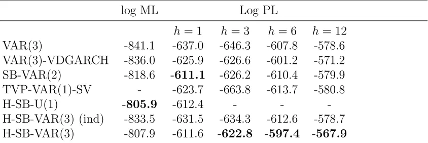
Figure 2 plots the posterior probability of structural change, P(dt = 1|Y1,T), over time

for the H-SB-VAR(1) model. It shows a strong pattern of parameter uncertainty. There are a significant number of breaks that are identified with over 0.8 probability.

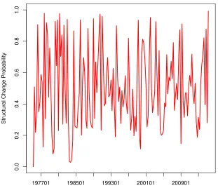
Figure 3 shows the data and in-sample posterior predictive means implied by the hierar-chical structural change model using the full sample. The top panel is the oil price change

7

and the bottom is the real GDP growth. The model that gives the best out-of-sample density forecasts also gives good in-sample fit.

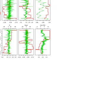
Figure 4 shows the standard deviations and the correlation coefficients of the error term over time for H-SB-VAR. The top panel and middle panel plot the standard deviations of the error terms of the oil price change and the real GDP growth, respectively. We can see a clear spike in 2008Q4, which coincides with the financial crisis. The correlation changes over time, however the deviations from zero, both positive and negative, are short lived. There is a large swing in 2008Q4 to 0.8 for the correlation coefficient, but it quickly reverts back to around zero.

7

A VAR for the U.S. Economy

In this application, we apply the structural break models to a medium size system with 7 variables downloaded from CITIBASE. They are: the unemployment rate (UR), Core PCE (1200×log difference of the level), nonfarm employment (1200×log difference of the level), retail sales (1200 × log difference of the level), housing starts level (100 × log difference of the level), industrial production index (1200 × log difference of the level), and the federal funds rate.8 There are 625 observations from 1959M02 to 2011M02. Summary statistics are shown in Table 3. We can notice that the variables are normalized differently from the variance column. This is not a problem since scaling is automatically corrected in the prior elicitation procedure. In the following we report results for models with a lag length that has the largest log-predictive likelihood. For all models a lag length from 1 to 4 is considered. The exception is for the H-SB-VAR specification in which lag lengths of 1 and 2 where estimated to reduce computation time.

Based on the H-SB-VAR model three features are discovered in this application. First, we find structural instability is an important feature for the U.S. macroeconomic variables, which is consistent with the literature. Second, volatility has a decreasing pattern in general, which is in line with the great moderation. However, some volatility jumps exist. Lastly, our approach finds the number of regimes is different from most of the current literature. Existing models either assume a small number of regimes (2 or 3) or structural change at each time (T). We find the best multivariate structural break model supports more than 5 regimes.

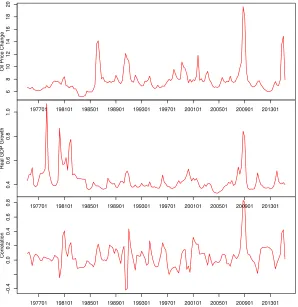
Figures 5 and 6 show the smoothed break probability over time for the SB-VAR and the H-SB-VAR models, respectively. The hierarchical model finds more than the two regimes identified by the non-hierarchical model. The SB-VAR has a relatively uninformative prior while the hierarchical model (H-SB-VAR) shrinks the prior towards something more plausible and hence breaks are needed to capture significant changes in the data. This results in improved forecasts that we discuss below.

Defining a break as the posterior break probability p(dt = 1|IT) > 0.5, the H-SB-VAR

model identifies 1960M06, 1979M10, 1982M12 and 2009M01 as the change-points. If using

p(dt = 1|IT) > 0.2 as the criteria of the structural change, 1979M09, 1984M03, 1987M12,

1995M05, 2001M01, 2001M11, 2007M12 and 2009M11 can also be considered as

change-8

points. This finding is consistent with Koop and Potter (2007) in their univariate analysis of U.S. GDP growth and inflation data.

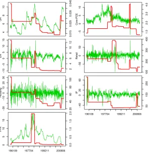
Figure 7 plots the posterior mean of φ(₁ii_,t) over time from the H-SB-VAR model. It represents the average effect of the first lag of the variable on itself. The unemployment rate (UR) and the federal fund rate (FFR) are very persistent for most of the time, while the rest of the variables are mean reverting. Figure 8 plots the posterior mean of the volatility

σ_t(i) of the innovations over time. All variables except Core PCE have a trend of decreasing volatility over time. The displayed parameter changes are not exactly the same as implied by the great moderation because heterogeneous dynamics exist for these macroeconomic variables. For example, some variables such as the unemployment rate and the federal fund rate had a volatility increase instead of a decrease after the 1979 break. Volatility of retail sales decreased after 1979, but after 1984M03 volatility jumped up. Industrial production had a volatility decrease after early 80’s; however, a volatility increase appeared during the most recent financial crisis.

Following a referee’s suggestion we compute the inflation gap persistence measure R2

t,h,

from Cogley et al. (2010).9 Whenh increases, a rapid decreasing ofR2_t,h towards zero means that most of the variation will be explained by the most recent shocks. This scenario implies weak persistence. If theR2

t,h converges to zero slowly, it shows strong persistence. A detailed

description can be found in Cogley et al. (2010). Figure 9 showsR2_t,h over time based on the multivariate hierarchical structural break model for horizonh= 1,3,6,12. We found the rate of decrease of persistence is quite fast in general. At h = 1, the persistence is already very low (around 0.2). And then it quickly drops to around 0.05 ath= 3. The model predicts the inflation persistence measured by the change of R2

t,h overh is quite low. Our results are not

the same as Cogley et al. (2010), who found time-varying inflation persistence. Because the density forecast do not favour the H-SB-VAR model, as discussed below, our results should be interpreted with caution.

The same set of comparison models as in the previous application are used in out-of-sample forecasts. Table 4 shows the predictive likelihoods and the root mean square forecast errors for the last 10 years (120 observations) of the sample. The second column is the predictive likelihoods. According to this the best VAR has a lag length of 4 and log-predictive likelihood of −1751.8. All structural break models significantly improve upon the VAR with log-predictive Bayes factors that range from 12.8 to 200. Note that adding the hierarchical prior to the SB-VAR model moves the log-predictive likelihood from−1695.6 to

−1551.8, a gain of 143.8.

The univariate hierarchical structural break specification (H-SB-U) has the best density forecasts.10 _{The log-predictive Bayes factor is 91.5 against the best multivariate} hierar-chical version and 143.8 against the non-hierarchical specification. Learning through the hierarchical structure is clearly important to improving density forecasts whether it be the multivariate or univariate model. The dominance of the univariate structural change spec-ification indicates that a more flexible change-point model which allows for asynchronous parameter change, may work better in the multivariate setting. Separate break processes

9

See the Appendix for the derivations of this measure.

10

appear to be more important than modeling contemporaneous correlations in the innova-tions. Similarly, the TVP-VAR-SV model is superior to the multivariate structural change models. Although the TVP-VAR-SV model has a separate evolution for each time-varying parameter and stochastic volatility for the conditional covariance matrix the application of the univariate structural break model to each series is substantially better with a log-Bayes factor of 32.7 in its favour.

Figure 10 displays the difference in cumulative log-predictive likelihoods for several mod-els against the benchmark VAR(4) model. The H-SB-U and TVP-VAR-SV are often close in the out-of-sample period but the performance of the former significantly improves around the financial crisis.

The remaining columns of the Table 4 report the root mean square forecast error of the predictive mean forecasts. The univariate structural change models often are the most accurate (4 out of 7 cases) but it can have poor performance when it is not. The VAR has the best point forecasts on Core PCE.

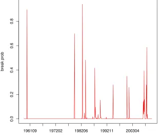
To see why the H-SB-U performs better than the multivariate structural change models, Figure 11 displays the posterior probability of a break for each series. These results are very different than Figure 6 in which all parameters must break at the same time. For the univariate models, except for Unemployment and Housing Starts all series display evidence of structural breaks but the frequency of breaks and the timing is very different. These results underscore the important of allowing for independent breaks in each data series and the impact this can have on forecasting.

8

Conclusion

A

Inverse Wishart - Matrix Normal prior

1. Σ:

The error covariance matrix Σ has a Inverse-Wishart distribution. Its prior mean is

E(Σ) = S

ν−N −1

The variance of each element

V ar(Σij) =

(ν−N + 1)S2_ij + (ν−N −1)S_iiS_jj

(ν−N)(ν−N −1)2_{(ν−N −3)}

Its density function is given by

p(Σ) = |S|

ν/2_|Σ|−_(ν+N+1)/2

etr{−1₂SΣ−₁

}

2νN/2_Γ

N(ν/2)

Γp is multivariate gamma function, which isΓp(a) =

R

S>0etr{−S}|S|

a−_(p+1)/2

dS where

S >0 meansSisp×ppositive definite matrix, or Γp(a) = πp(p−1)/4Qp_j=1Γ(a+(1−j)/2)

A special case is when N = 1. Then Σ =σ2 _{as a scalar and}

p(σ2) = s

ν/2_(σ2₎−_ν/2−₁

exp{−s₂σ−₂ }

2ν/2_Γ(ν/2) .

So σ2 _{has an inverse-gamma distribution with a shape parameter ν/2 and a scale} parameter ₂s. The mean and the variance of the σ2 _{equal to} s

ν−₂ and

2s2

(ν−₂₎2_(ν−₄₎,

respectively.

The precision matrixP, which is the inverse of the covariance matrix Σ, has a Wishart distribution W(P , ν), where P =S−₁

. It has density

p(P) = |P|

−_ν/2

|P|(ν−_N−_1)/2

etr{−1₂P−₁

P}

2νN/2_Γ

N(ν/2)

A special case is when N = 1, then P =σ−₂

has a gamma distribution with

p(σ−2

) = s

ν/2_(σ−₂

)ν/2−₁

exp{−s₂σ−₂ }

2ν/2_Γ(ν/2) .

The mean and variance of σ−₂

are ν_s and 2_sν2.

2. Φ:

The regression coefficient matrix Φ has a matrix normal distribution. Each column of Φ, Φ.j, is the regression coefficients for thejth equation and has a multivariate normal

distribution

Each row of Φ, Φi., is the coefficients of impact from the same source across equations.

Φi.|Σ∼N(Φi.,ΣΩii)

The density function is

p(Φ|Σ) = etr{−

1 2Σ

−1

(Φ−Φ)′

Ω−1

(Φ−Φ)}

(2π)M N/2_|Σ|M/2_|Ω|N/2

B

Sample from a matrix Gaussian

For Φ|Σ ∼ M N(Φ,Σ⊗Ω), to generate a sample of Φ, first get lower triangular matrices Σ1/2 _{and Ω}1/2 _{through Cholesky decomposition. Then, generate C ∼ M N(0, I ⊗I). Φ is} generated from

Φ = Ω1/2CΣ1/2′,

since vec(Ω1/2CΣ1/2′

) = Σ1/2_⊗Ω1/2_{vec(C). So the variance of vec(C) is Σ}1/2_⊗Ω1/2_(Σ1/2_⊗ Ω1/2)′

= Σ1/2_⊗Ω1/2_(Σ1/2′

⊗Ω1/2′) = (Σ1/2_Σ1/2′

)⊗(Ω1/2Ω1/2′) = Σ⊗Ω

C

Sample from an Inverse-Wishart distribution

Generate Σ from a Inverse-Wishart, IW(S, ν), by

Σ =S1/2C−₁

S1/2′

where S1/2 is the lower triangular matrix from the Cholesky decomposition of S and C is drawn from a Wishart W(I, ν).

D

Sample the hierarchical prior

1. Φand Ω:

The prior is matrix normal and inverse-Wishart.

Ω∼IW(Ω0, ω0) Φ|Ω∼M N(M0,Λ0⊗Ω)

The conditional posteriorΦ,Ω|{Σi,Φi}Ki=1 is

Ω|{Σi,Φi}iK=1 ∼IW(Ω1, ω1) Φ|Ω,{Σi,Φi}iK=1 ∼M N(M1,Λ1⊗Ω)

with

Ω1 = Ω0+

K

X

i=1 ΦiΣ

−₁ i Φ

′

i+M0Λ −₁

0 M

′

0−M1Λ

−₁

1 M

′

ω1 =ω0 +KN

M1 = (M0Λ

−1

0 +

K

X

i=1 ΦiΣ

−1 i )Λ1

Λ1 = (Λ−1

0 +

K

X

i=1 Σ−1

i ) −1

2. S:

The prior of S is a Wishart W(S0, τ0). The conditional posterior is also Wishart.

S|ν,{Σi}K_i=1 ∼W(S1, τ1)

with

S−₁

1 =S

−₁

0 +

K

X

i=1 Σ−₁

i

τ1 =τ0+Kν

3. ν:

The prior is a Gamma G(a0, b0). The conditional posterior has no convenient form.

p(ν|S,{Σi}Ki=1) =pG(ν;a0, b0)

K

Y

i=1

p(Σi|S, ν)

∝pG(ν;a0, b0)

K

Y

i=1

|S|ν/2 2νN/2_Γ

N(ν/2) |Σi|−

ν+N+1 2

∝νa0−1

e−b₀ν |S|

Kν/2

2KνN/2_ΓK N(ν/2)

K

Y

i=1

n

|Σi|−ν+N+1

2

o

The log of the last equation (after discarding more constants) is

Klog(|S|)−2b0−KNlog(2)−PK_i=1log(|Σi|)

2 ν−Klog(ΓN(ν/2)) + (a0−1) log(ν).

The sampling method of ν is a M-H step with a proposal distribution of

ν(i) ∼G(ξ, ξ/ν(i−1)

)

E

VAR-VDGARCH Prior

2. The prior of a and b is given by the following transformation

a= e

θ1

1 +eθ1 +eθ2, b=

eθ2

1 +eθ1 +eθ2

We set the mean of θ1 and θ2 to satisfy a = 0.2 and b = 0.7. The prior of θ1 and θ2 are assumed to have normal distributions with the aforementioned mean and variance of 10.

3. The prior of C is set as normal distribution with the following parametrization:

(a) Let the stationary covariance matrix H = CC′

1−_a−_b equals to the prior mean of the

covariance matrix in the VAR model, wherea and b are set as their prior means. SolveC by using Cholesky decomposition.

(b) Take log of the diagonal elements of C and vectorize the lower triangular of C

(notice thatC is a lower triagular matrix). This vector is set as the prior mean. (c) The covariance matrix is set as 10 times an identity matrix.

F

MCMC for independent break chains

1. Sample DΦ_,Φ|DΣ_{,Σ, π}

Φ, πΣ,Φ,Ω, S, ν, Y1,T, X1,T.

From (9), the conditional density of yt is

yt | · ∼N(Φ ′ txt,Σt)

If there is no break at time t, the conditional posterior Φt|dΦt−₁ =d, Y1,t−₁,·is

p(Φt|dΦt−₁ =d,·)

∝etr

−1

2[vec(Φt)−vec(Φ)]

′

(Σ∗

⊗Ω)−1

[vec(Φt)−vec(Φ)]

×etr ( −1 2 d X i=1

(yt−i−Φ ′ txt−i)

′

Σ−₁

t−_i(yt−i−Φ ′ txt−i)

)

Let’s focus on the terms inside the etr operator and discard the multiplier −1 2 for notational simplicity.

[vec(Φt)−vec(Φ)] ′

(Σ∗

⊗Ω)−₁

[vec(Φt)−vec(Φ)] + d

X

i=1

(yt−_i−Φ ′ txt−_i)

′

Σ−₁

t−_i(yt−_i−Φ ′ txt−_i)

=vec(Φt) ′

(Σ∗

⊗Ω)−₁

vec(Φt)−2vec(Φ)

′

(Σ∗

⊗Ω)−₁

vec(Φt) +const

+

d

X

i=1

vec(Φt)

′

Σ−₁

t−_i⊗xt−_ix ′ t−_i

vec(Φt)−2

d

X

i=1 (y′

t−_iΣ −₁ t−_i)⊗x

′ t−_i

vec(Φt) +const

=vec(Φt) ′

(Σ∗

)−₁

⊗Ω−₁

+

d

X

i=1 Σ−₁

t−_i⊗xt−_ix ′ t−_i

!

−2

"

vec(Φ)′

(Σ∗

)−₁

⊗Ω−₁

+

d

X

i=1 (y′

t−_iΣ −₁ t−_i)⊗x

′ t−_i

#

vec(Φt)

Hence

vec(Φt)|DΦt−₁ =d,· ∼N(m, H

−₁

),

whereH = (Σ∗

)−₁ ⊗Ω−₁

+

d

P

i=1 Σ−₁

t−_i⊗xt−_ix ′ t−_i

andm=H−1

"

((Σ∗

)−₁

⊗Ω−₁

)vec(Φ)+

d

P

i=1 (Σ−1

t−iyt−i)⊗xt−i

#

Suppose that if there is no structural change, the conditional data density ofyt is

yt |Φt, dΦt =d+ 1,· ∼N((IN ⊗x

′

t)vec(Φt),Σt)

Integrating out Φt, we have

yt |dΦt =d+ 1,· ∼N((IN ⊗x

′

t)m,(IN ⊗x ′ t)H

−₁

(IN ⊗xt) + Σt)

Now we can draw DΦ _{first and then draw Φ| D}Φ _{by applying the same technique in} this paper.

2. Sample DΣ_,Σ|DΦ_{,Φ, π}

Φ, πΣ,Φ,Ω, S, ν, Y1,T, X1,T

If there is no structural change ar time t, the conditional posterior Σt|dΣt−₁ =d, Y1,t−₁

is

Σt |dΣt−1 =d, Y1,t−₁,· ∼IW(S, ν),

where ν=ν+d and S=S+

d

P

i=1

(yt−_i−Φ ′

t−_ixt−_i)(y_t−_i−Φ ′

t−_ixt−_i) ′

.

The conditional data density ofyt is

yt |Σt, dΦt =d+ 1,· ∼N(Φ

′ txt,Σt)

Integrating out Σt, we have

yt |dΦt =d+ 1 ∼t

Φ′ txt,

S

v+ 1−N, v+ 1−N

,

with variance S/(v−N −1).

Now we can draw DΣ _{first and then draw Σ| D}Σ _{by applying the same technique in} this paper.

3. Sample πΦ |DΦ.

Assume that the prior πΦ ∼B(πaΦ, πbΦ). Similar to the nonhierarchical model, draw

πΦ |DΦ ∼B(πΦa +KΦ−1, πbΦ+T −KΦ),

4. Sample πΣ |DΣ.

Assume that the prior πΣ ∼B(πaΣ, πbΣ). Similar to the nonhierarchical model, draw

πΣ |DΣ ∼B(πΣa +KΣ−1, πbΣ+T −KΣ),

where KΣ is the total number of change-points of Σ.

5. Sample Φ,Ω|DΦ_{, D}Σ_,Φ,Σ

The prior is matrix normal and inverse-Wishart.

Ω∼IW(Ω0, ω0) Φ|Ω∼M N(M0,Λ0⊗Ω)

Suppose there are K regimes and each regime has distinct value Φ∗

i. The conditional

posterior Φ,Ω|{Φ∗ i}Ki=1 is Ω|{Φ∗

i}Ki=1 ∼IW(Ω1, ω1) Φ|Ω,{Φ∗

i}Ki=1 ∼M N(M1,Λ1⊗Ω) with

Ω1 = Ω0+

K

X

i=1 Φi(Σ

∗

)−₁

Φ′

i+M0Λ −₁

0 M

′

0−M1Λ

−₁

1 M

′

1

ω1 =ω0 +KN

M1 = (M0Λ−01 +

K

X

i=1

Φi(Σ∗)−1)Λ1

Λ1 = (Λ−₁

0 +K(Σ

∗

)−₁

)−₁

6. Sample S|DΦ_{, D}Σ_{, ν,Φ,Σ. Same as the hierarchical model.}

7. Sample ν|DΦ_{, D}Σ_{, S,Φ,Σ. Same as the hierarchical model.}

G

Inflation Persistence

Briefly, we start from Equation (9) and focus on its VAR representation by using notations similar to Cogley et al. (2010):

zt=µt+Atzt−₁+e_t, e_t∼N(0,Σ_t), (41)

where zt includes current and lagged values of yt. The vector µt is the intercept and At

represents the autoregressive coefficients.11

Conditional on At, assuming stationarity and no structural change afterwards, the

con-ditional mean of zt is denoted as

zt= (I−At)

−₁

µt (42)

The inflation gap can be written as

(zt−zt) = At(zt−₁−z_t) +e_t (43)

A h-period ahead forecast of the gap has variance

vart(ˆzt+h) = h−₁

X

j=0

Ajtvar(et)(Ajt)

′

=

h−₁

X

j=0

AjtΣt(Ajt)

′

(44)

If no previous shocks are observed, the forecast variance of the gap is equivalent to the case when h→ ∞:

var(ˆzt+h) = ∞

X

j=0

AjtΣt(Ajt)

′

(45)

Cogley et al. (2010) proposed an R2 _{type statistic to measure inflation gap persistence.} Specifically,

R2_t,h = 1− vart(eπzˆt+h)

var(eπzˆt+h)

= 1−

eπ

"

h−1

P

j=0

Aj_tΣt(Ajt)

′

#

e′ π

eπ

"

∞

P

j=0

AjtΣt(Ajt)′

#

e′ π

, (46)

whereeπ is a selection vector for inflation gap. Whenh increases, a rapid decreasing ofR2t,h

towards zero means that most of the variation will be explained by the most recent shocks. This scenario implies weak persistence. If the R2

t,h converges to zero slowly, it shows strong

persistence. A detailed description can be found in Cogley et al. (2010).

11

We illustrate with SB-VAR(1) as an example. Equation (9) can be written as

yt=µt+Atyt−1+et; et∼N(0,Σt),

with Φ′

t= (µt, At). We draw Φt from the posterior without imposing stationarity restrictions. Hence, no

References

Banbura, M., Giannone, D., and Reichlin, L. Large bayesian vector auto regressions. Journal of Applied Econometrics, 25(1):71–92, 2010.

Baumeister, Christiane and Kilian, Lutz. Forecasting the real price of oil in a changing world: A forecast combination approach. Journal of Business & Economic Statistics, 33 (3):338–351, 2015.

Baumeister, Christiane and Peersman, Gert. The role of time-varying price elasticities in accounting for volatility changes in the crude oil market.Journal of Applied Econometrics, 28(7):1087–1109, 2013.

Bauwens, Luc, Carpantier, Jean-Franois, and Dufays, Arnaud. Autoregressive moving aver-age infinite hidden markov-switching models. Journal of Business & Economic Statistics, 35(2):162–182, 2017.

Belmonte, M., Koop, G., and Korobilis, D. Hierarchical shrinkage in time-varying parameter models. Journal of Forecasting, 33(1):80–94, 2014.

Carriero, Andrea, Clark, Todd E, and Marcellino, Massimiliano. Bayesian vars: specification choices and forecast accuracy. Journal of Applied Econometrics, 30(1):46–73, 2015.

Casella, G. and Robert, C.P. Rao-Blackwellisation of sampling schemes. Biometrika, 83(1): 81, 1996.

Chib, S. Estimation and comparison of multiple change-point models. Journal of Econo-metrics, 86(2):221–241, 1998.

Clark, T.E. and McCracken, M.W. Averaging forecasts from vars with uncertain instabilities.

Journal of Applied Econometrics, 25(1):5–29, 2010.

Cogley, T. and Sargent, T.J. Drifts and volatilities: monetary policies and outcomes in the post WWII US. Review of Economic Dynamics, 8(2):262–302, 2005