Fiscal policy in developing countries: Do governments wish to have procyclical fiscal reactions?

Munich Personal RePEc Archive

Fiscal policy in developing countries: Do

governments wish to have procyclical

fiscal reactions?

GBATO, ANDRE

CERDI

19 August 2017

Online at

https://mpra.ub.uni-muenchen.de/80881/

Fiscal policy in developing countries: Do governments wish to have

procyclical fiscal reactions?

André GBATO1

Abstract:

This study aimed to analyze the intentionally fiscal position of the governments of developing

countries. Our results suggest that a significant proportion of developing countries adopts

counter-cyclical positions. However, forecasting errors weak their positions. Results lead to

conclude that if developing countries want to increase the effectiveness of their fiscal policies,

they must build the skills of their forecast offices, and enhance the political and institutional

framework governing the budget process.

Keywords: Fiscal policy; Real Time Data; Developing countries; Generalized moment

method, revision errors

JEL Classication System: C23, E30, E62, H30, H60

1

I.

Introduction

The recent crisis of 2008 has led to a renewed interest in Keynesian policies.Faced with the

global downturn, the cyclical policies were seen as a remedy capable of restoring

growth.There is recent empirical evidence that developed countries have intentionally

designed countercyclical policies.This implies that these states were sympathetic, since the

purpose of such policies is to support economic activity.In developing countries, however,

few studies have asked about the real intentions of governments in terms of fiscal policies.If

intentional, governments of developing countries have implemented pro-cyclical policies

would mean that they are ill-disposed to the image of "Leviathan" presented by political

economy.The question is to know which policies were designed.Have the governments

designed procyclical or countercyclical policies?

According to the literature, fiscal policy was pro-cyclical in all developing

countries(Gavin and Perotti, 1997;Agenor, McDermott and Prasad, 1999;Kaminsky,

Reinhart and Végh, 2004).Based on this result, it is generally accepted that the procyclicality

would consciously desired by policymakers for electoral reasons.However, the lessons

learned from work on the behavior of the monetary authorities could lead us to question the

validity of such a belief.

The common point of the previous studies is the use of revised data.If these studies are

effective in determining the meaning "in fine" of fiscal policy, they are not suitable for

assessing the budgetary position "real" or intentional government(Orphanides, 2001;Forni

and Momigliano, 2004;Cimadomo, 2008).The analysis of the government's position should

be based on the information available to decision makers in real time.The position of the

State could thus be understood by stakeholder changes in the budget in year t + 1, following

the conditions in year t to which the government faces.However, previous studies have

privileged data that revisions can be significant (see graph 1).The main consequence of these

revisions is that the value of GDP could be different from one year to another.Now,

governments are accustomed to adopt their position relative to their perception of the output

gap2. This implies that if at time t the government increases spending following a negative

gap in real time, a revision of GDP ex-post that would lead to a positive gap would lead to a

finding of procyclical behavior of government.In this context, analyze the position of States

on the revised database could be problematic because the position they would suggest, the

2

result could be "in fine" of institutional and macroeconomic factors, but not necessarily the

intention of government.This implies that the role assigned to governments could be only

a "non-sequitur."Another formulation of the problem may emerge if we look at the

implication of the use of revised data.If the objective is to study the behavior of the

government, the use of revised data implies an assumption of high availability.Indeed, this

implies that the data available to the researcher are the same as those available to the

government.However, as confirmed in Chart 1, this assumption is not always true.

Moreover, the difficulties associated with forecasting exercises developing countries have

rarely been seen in previous models.Yet these difficulties have been identified in the

literature as additional constraints to the implementation of fiscal policy (IMF, 2010)3. Few

studies to our knowledge have examined the role of forecast errors on the position of

governments.However, such a study could tell us more about the behavior of states. It would

be important to know why government's position is often procyclical to design a better policy

reaction.

In this study, we follow the approach ofBernoth, Hughes and Lewis (2008)to determine the

position of the government and the impact of forecast errors.According to the arguments

ofKaminsky, Reinhart and Végh, 2004andLledó, Yackovlev and Gadenne (2011),we

analyze the position of the State from the total expenditure.In addition, we correct the

possible endogeneity bias by using the generalized method of moments.

The article is organized as follows: Section 1 highlights the concept of real-time analysis and

measurement, section 2 provides an overview of the literature on the position of States, and

the final section presents the applied analysis.

II.

ANALYSIS IN REAL TIME

1. Concept

The real-time analysis recently appeared in empirical work on monetary policy.This approach

was implemented byOrphanides (2001),to investigate the robustness of the policy

recommendations in the area of monetary authorities in the United States.In his study, he

showed that when unrealistic assumptions about the data are made available opportunity,

especially when it is assumed that the information updated and revised previously are

3

available to policy makers, behavior analysis politicians can lead to misleading results.Since

this approach has opened new avenues of research and helped many works.

The concept of real-time analysis or "Real Data" is based on exploration data available to

decision makers at the time of decision making.These data are distinguished in the literature

by the name of data "ex-ante".The revised data are for their data called "ex-post".

The uses of ex-ante budget analysis data in reports to a particular frame.During the financial

year (t) are tabulated resources and expenditure.Based on these figures, the government

conducts a screening of these indicators to the end of the year, and designs its objectives of

revenue and expenditure for the next fiscal year (t + 1).These objectives are then included in

the draft Finance Act, which will be submitted to the vote of Parliament.

As part of our study, we will use as a proxy for ex-ante governments GDP, GDP in the current

year, published in each version of the IMF WEO4. This choice is justified by the fact that

most of the WEO projections are the result of discussions, during which the IMF staff and

national authorities agree on the projection assumptions for the end of the current year and for

the following year.On many consultations5 relating to several countries, we have not observed significant differences between the projections of the IMF and the national

authorities.Instead, the IMF figures vary in the same direction as the national

figures.Moreover, the IMF WEO database provides a uniform and consistent measure of

output, which alleviates the differences in national accounting.Finally, accordingLledo and

Pibeiro-Poplawski (2011)these data are very reliable because they embody the best estimates

of the IMF plans and feasible viable national authorities, even though they do not always

reflect their views in full6.

2. Notation

The use of real-time analysis uses a special notation. Let t represents time (Annual or

Monthly), and V any variable. It is commonly accepted the following notation: ,

which defined the value of the variable V to the period which is provided for the period

. If , corresponds to a forecast. If , corresponds to the real time value,

4

Hughes and Lewis used a similar method in the OECD. Poplawski-Ribeiro and Lledo (2013) use the same method for sub-Saharan Africa

5

Consultations under Article IV country reports produced by the IMF

6

in the sense that it is the latter which is available to the decision-maker. If ,

corresponds to the value of the variable published years after the event (revised). Note that is

a natural number.

III.

Literary and temperature

Fiscal policy has given rise to numerous empirical studies. In developing countries, there is a

consensus on the procyclicality of fiscal policy, primarily based on ex-post data. Gavin and

Perotti (1997) were the first to draw attention to the fact that tax policy Latin America seems

average procyclical, with recessions are associated with exaggerated collapses in public

expenditure. This result is confirmed by Stein, Talvi, and Grisanti (1999), who find a way

correlation coefficient of 0.52 between the cyclical component of public consumption and the

cyclical component of production over the period 1970-1995 for sample of 26 Latin American

countries. Similarly, from a sample of 36 developing countries from Asia, Africa, the Middle

East, and Latin America Talvi and Carlos Vegh (2000) find that public consumption is very

pro-cyclical, with a correlation coefficient of 0.53. However, Agenor, McDermott and Prasad

(1999) note that government consumption expenditures countercyclical for a group of four

middle-income countries i.e. Chile, Korea, Mexico and the Philippines.

Kaminsky, Graciela, Reinhart, and Végh (2004) will re-evaluate fiscal policy in developing

countries. They find that fiscal policy is procyclical in their sub-sample of 83 low-income

countries and middle income. This will be confirmed by Akitoby, Clements, Gupta and

Inchauste (2004).

Furthermore, Empirical studies suggest that the introduction of a countercyclical policy would

face several factors. The various budget stages and the race for power of different political

factions (Buchanan and Wagner, 1977; Lane and Tornell, 1996, 1999; Woo, 2003a, b,

2005; Hallerberg, Strauch and von Hagen, 2004), difficulties in evaluation of real cycles

leading to lags in the selection and implementation of fiscal policy (Akitoby et al, 2004), the

low share of transfer expenditures reducing the scope of the automatic stabilizers (Lane,

2003b), financial constraints and limited access to capital markets, are all reasons that can

lead to a procyclical fiscal policy (Gavin and Perotti, 1997; Kaminsky et al., 2004)7. When

discretionary action results in a pro-cyclical stance, these factors are likely to amplify

economic fluctuations.

7

It appears from this literature review that previous work did not provide concrete evidence of

the willingness of the government. There is only that suspicions, based primarily on the use of

ex-post data. In the next section, we present an analytical framework to mitigate potential bias

related to data availability hypothesis before proceeding with an econometric estimation.

IV.

APPLIED ANALYSIS

1. Determination of output

A consequence of the time analysis is that the estimate of the output can now be done directly

from the revised GDP data.The government decided to adopt the position that according to

the evolution of output (Output gap) and the level of fiscal indicators.However, it does not

have the revised data as they present themselves today.To retrieve the output in real time, we

must first identify the part of the final data due to revisions.Thus, the problem can be

formalized according Bernoth, Hughes and Lewis (2008) by decomposing the GDP (Y) as

follows:

(1)

With potential value of GDP and output gap.No revisions data of each vintage would

be the same.The various revisions therefore imply that:

(2)

(3)

With GDP of year estimated at the year , the latest available GDP. is the potential value of GDP calculated on the basis of the information available at ,

the gap between GDP in real-time and final GDP and the gap between potential output

in real time and the final potential GDP.

Finally, the combination of equations (1) (2) and (3) allows the output estimated in real time

based on the final GDP and different deviations implied revisions:

(4)

(5)

Knowing that the latest version (i.e.t+s _{= f) isa given and that only vary the data of previous}

vintages, equation (6) implies that the gap in real time and the difference between the gaps

move in the same direction.

2. Construction of fiscal reaction function

The study discretionary policies require a model to capture the variations of fiscal indicator

compared to the production space (output gap).Most empirical studies use the budget

balance (SB

) as the dependent variable and a set of control variables (

models used adopt the following form:

(7)

In this form, however, this model has some shortcomings:

1. First, the use of the budgetary balance may be problematic in the context of sub-Saharan African countries, and in particular in the case of UEMOA countries.

These countries are heavily dependent on external resource flows. These flows are

unstable. As a result, the level of resources and the overall balance do not always

correspond to the will of public decision-makers (Kaminsky, Reinhart and Vegh, 2004; Lledo et al., 2009).

2. Then, this model is designed to exploit ex-post data information. But, as

mentioned above, these data lead to a bias in the results.

To overcome the first problem,Kaminsky, Graciela, Reinhart, and Végh (2004)andLledó,

Yackovlev, and Gadenne (2011)advocate the use of government spending instead of the

budget balance.They argue that in developing countries, spending is more telling of the will

of the state.

Regarding the second problem,Forni and Momigliano (2004) and Cimadomo (2008)equation

is entirely based on the data in real time:

(8)

Their intuition is that the government provides its position according to real-time conditions.In this model, the fiscal balance ( ) is adjusted for its cyclical variation, and the

government's position is captured by the sign . So if fiscal policy is

countercyclical;otherwise it is procyclical.But if , fiscal policy is acyclic.However, two observations can be made. The first point is that the equation (8) is responsive to the correction of the cyclic variations in tool.In the case of the use of Prescott filter, the

of fiscal indicators would be hazardous in sub-Saharan Africa (Lledó, Yackovlev, and

Gadenne, 2011).The second is that the level in real time in the dependent variable might just

match what was recorded, not necessarily to decision makers (Hughes et al, 2008).

For all these reasons, we proceed as Hughes et al (2008) to establish reaction function

operator information ex post data while mitigating through revision.The starting point of the

model is the assumption that the budget ( ) is responsive to three elements. First, a portion of

the budget is supposed to automatically respond at the current production.This hypothesis is

that several studies argue that automatic stabilizer ( ) plays a role in developing

countries(Chami, Hakura and Montiel, 2009; Suescun, Rodrigo, 2007; Debrun and

Kapoor, 2010).

Then let some work believe that part of the budget would depend on potential output.For

example, incentives for international technical assistance to increase the tax burden where to cut spending often based on the exploration of potential GDP.Thus, parameter capture

discretionary changes following potential GDP.

Finally, the government adopts its position based on its perception of the production

space.Therefore captures the discretionary state action.So we have:

(9)

When the data used are those for the latest year available, we have:

(10)

Substituting (2) and (3) in (9), and one obtains:

(11)

Equation (11) means that the real position of the government may be captured by the sign of

.It also means that fiscal policy is based on differences between ex-ante and ex-post values

of potential GDP.This equation also suggests that the coefficient of ex-post gap is composed

of the position of the State and the impact of automatic stabilizers.Finally, we express all

variables in ratio of final potential GDP to avoid any problems of measures and minimize the

influence of ex-ante GDP8, we get:

(12)

8

(13)

3. Estimation Method

To effectively capture the decision makers, we estimate the following equations:

(14)

(15)

Where the vector Ԑ idiosyncratic errors, is a vector of relevant variables considered in the

literature.We introduce the control variables from the public debt, which allows the level of

spending lagged to take account of initial conditions.

We begin our analysis by pooling test.We find that the P-value of Fisher test is below the 5%

threshold.We therefore conclude that there are fixed effects.We then apply the unit root test

of Im, Pesaran and Shin (2003).For lags of 1 to 3, we find a lower P-value to the significance

level.This implies that our variables are stationary and therefore do not need to be

differentiated to perform regressions.

The presence of the lagged dependent variable in our model implies that the OLS estimator is

not consistent.The literature in this case recommends the use of the generalized method of

moments (GMM).We use the system GMM estimator of Blundell and Bond (1998), which

uses lagged differences of the dependent variable as instruments of level equations and level

lagged variables as instruments of difference equations.According to these authors, this

estimator significantly improves the performance of the estimator in difference of Arellano

and Bond (1991).Moreover, Bun and Kiviet (2006) and Hayakawa (2007)show that face a

dynamic panel, where the individual and temporal dimensions are finished, the system GMM

estimator is a safe choice compared to the estimator in difference of Arellano and Bond

(1991)9.

The results of the GMM are validated by three conditions.Must be an adequate number of

lags, because a large number of lags reduces significance of Hansen identification test.In

addition, for the building GMM involves the autocorrelation of the first order, the results are

only relevant if there is no autocorrelation of order 2. Another important point is that the

number of instruments should be less than the number of sample observation.Finally, the

choice of the endogenous variable or not affects the quality of results.Next Kiviet and Bun

(2006) and Hughes et al (2008), we choose to limit to three the number of lags in the level

equations and difference.We consider the variables v, z and lagged expenditures (dep) as

weakly endogenous and debt as endogenous in all equations.

9

4. Descriptive Analysis

The table (1) presents the descriptive statistics of our key variables.The average debt and spending, and their dispersion seem relatively low.By cons, very high average is observed

and a very strong dispersion for goodwill estimate of potential GDP (v) and the output gap

(z).These high numbers may partly be explained by the revision of the calculation of

GDP.Some countries have revised their method of calculating GDP, which led to strong

upward revisions of GDP.Certainly, this type of review is not really a mistake, but for our

purposes we assimilate to the GDP estimation error.This choice can be justified by the fact

that if these changes had occurred at the time of the catch of past positions, the government's

behavior would not have been the same.In addition, a new calculation suggests that the old

way was not sufficiently representative of reality, and therefore was more likely to be

misleading.

We build two graphs(Graph 1 and Graph 2)representing the evolution of expenditure

respectively from the output then compared to ex-ante and ex-post differences in potential

GDP.The two graphs confirm the strong dispersion of the variables in the output gap ex ante

and the error associated with the estimate of potential GDP.Furthermore, Graph 1 shows a

downward trend, implying that an increase in the output gap is followed by reduction of final

expenditure. As against the Graph 2 shows an upward trend, which implies that expenses are

moving in the same direction as the estimation of potential output errors.

Graph 1: Expenditure in relation to ex-ante gap Graph 2: Expenditure compared to forecast errors of potential GDP

0 20 40 60 80 1 0 0

-20 -10 0 10 20 30

Output gap ex-ante

Dépenses ex-post 90% CI Fitted values 0 20 40 60 80 1 0 0

-100 -50 0 50

Ecart PIB potentiel ex-ante et ex-post

5. Estimates of the position of governments

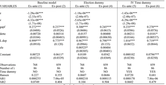
Table (2)shows the results of the estimation in GMM system.To test the robustness of our

results, we first include a dummy variable (ele) representative election years.We hope to

capture the influence of electoral cycles.Overall the results remain the same in columns (3)

and (4). We then perform our regressions using as instrument the time fixed effects.Intuition

is to capture the influence of exogenous shocks that may have influenced the willingness of

governments during the period.We find similar results in columns (5) and (6).

It is noted that the lagged expenses are significantly positive in all columns, while the debt is

not significant.This underlines the importance of the level of spending in the decision making

process in accordance with the literature.The insignificance of debt contrary to the

predictions of the literature could be explained by the substantial debt reductions that

benefited a number of developing countries

In columns (1), (3) and (5), the government's position (z) is significantly negative. These results mean that developing countries generally have designed countercyclical policies over

the period. Regarding the forecast errors of potential GDP (v), we see that they are

significantly negative. These results mean that the forecast errors of potential GDP have reduced spending.This implies that the government's reaction has been reduced below the

optimal level over the period.

In all columns, we find that the final output gap is significantly positive.Referring to equation

(11), this means that the automatic stabilizers have had a positive impact on spending. This

result could be explained by weak institutions in developing countries, according to the

literature that may affect the operation of automatic stabilizers.

V.

Conclusion

This study aimed to define the desired position intentionally by the governments of

developing countries.This analysis was based on recent literature data in real time.To achieve

our goal, we first conduct a theoretical analysis of the composition of the output gap, and we

have built a fiscal reaction function for capturing the intentional government position.

Our results suggest that a significant proportion of developing countries have adopted

counter-cyclical positions. However, errors in assessments of potential GDP contribute to

weak their positions. In other words, these governments have desired implement

countercyclical policies, but have been misled by an incorrect assessment of their potential

GDP.

Overall, these results are perplexing as to the effectiveness of fiscal policies.Indeed, although

outcome of procyclical policies is found in most studies.This leads us to believe that the

causes mentioned in the literature probably prevent the stabilization budgetary measures so

that their performances are not made on time, or not do against the economic cycle.

Finally, this study leads to think that if developing countries want to increase the effectiveness

of their policies, they must build the skills of their forecast offices, and enhance the political

REFERENCES

Agenor, PR, McDermott, J., and Prasad, ES, 1999. "Macroeconomic Fluctuations in

Developing Countries: Some Stylized Facts," IMF Working Paper 99/35 (Washington:

International Monetary Fund).

Akitoby, B., B. Clements, Gupta and G. Inchauste S. (2004) 'The Cyclical and Long-Term

Behavior of Government Expenditures in Developing Countries', International Monetary

Fund, Working Paper No. WP / 04/202.

Andrews (2010), "How far public financial management-have come Reforms in Africa?"

Research Working paper RWP10-018.Cambridge: Harvard Kennedy School

Arellano, M. and O. Bover (1995), "Another look at the instrumental variable estimation of

error-components models", Journal of Econometrics, No.68, 29-52.

Beetsma, Giuliodori, & Wierts (2009), Planning to cheat: EU tax policy in real time,

Economic Policy, 60 (2009), pp.753-804

Blundell, R. and S. Bond (1998), "Initial requirements and time restrictions in dynamic panel

data model", Journal of Econometrics, No.87, 115-143.

Ralph Chami, and Dalia Hakura Montiel, Peter (2009) Remittances: An automatic stabilizer

output ?, IMF Working Papers.Available at SSRN: http://ssrn.com/abstract=1394811

Carmignani (2010), "Cyclical fiscal policy in Africa", Journal of Policy Modeling, 32 (2010),

pp.254-267

Cimadomo (2008), "Fiscal policy in real time", European Central Bank, Working Paper Series

0919

Cimadomo (2011), "Real-time data and fiscal policy analysis: a survey of the literature"

Working Paper Series 11-25, Federal Reserve Bank of Philadelphia

Forni, M. and S. Momigliano (2004), "Cyclical sensitivity of fiscal policies were based

real-time data," Applied Economics Quarterly 50

Gavin, M. and R. Perotti (1997), "Fiscal Policy in Latin America", in B. Bernanke and

Rotemberg J. (eds), NBER Macroeconomics Annual 12, Cambridge, MA: MIT Press, pp.

11-70.

Ilzetzki & Vegh (2008), "Tax policy in developing countries Procyclical: Truth or fiction"

Im, K., H. Pesaran, and Y. Shin (2003), "Testing for Unit Roots in Heterogeneous Panels",

Journal of Econometrics 115, 53-74.

John Thornton (2008), "Explaining Procyclical Fiscal Policy in African Countries" Journal of

African Economies, Volume 17, No. 3, pp. 451-464

Kaminsky, Graciela, Carmen Reinhart and Carlos A. Vegh, 2004, "When It Rains, It Pours:

Procyclical Capital Flows and Macroeconomic Policies," in NBER Macroeconomics

Annual, ed. by Kenneth Rogoff and Mark Gertler (Cambridge, MA: MIT Press).

Kerstin Bernoth, Andrew Hughes Hallett and John Lewis (2008), "Did tax policy makers

know what They Were doing? Reassessing tax policy with real-time data ", De Nederlandsche

Bank., Working Paper No. 169

Orphanides, A. (2001), "Monetary Policy Rules Based on Real-Time Data", American

Economic Review, No.91, 964-985.

Ernesto Stein, Ernesto Talvi, and Alejandro Grisanti, 1999 "Institutional Arrangements and

Fiscal Performance: The Latin American Experience," NBER Working Paper No. 6358

Suescun Rodrigo, Size and Effectiveness of Automatic Fiscal Stabilizers in Latin America (June 1, 2007). World Bank Policy Research Working Paper No. 4244. Available at SSRN: http://ssrn.com/abstract=991436

Carlos Ernesto Talvi and Végh, 2000 "Tax Base Procyclical Variability and Fiscal Policy,"

NBER Working Paper 7499 (Cambridge, MA: National Bureau of Economic Research).

Victor Lledó, Irene Yackovlev, and Lucie Gadenne (2011), "A Tale of Procyclicality, Aid and

Debt Flows: Government Spending in Sub-Saharan Africa", African Journal of Economics,

20 (5), 823-849

Victor Lledo, and Marcos Poplawski-Pibeiro (2011) Fiscal policy implementation in

Sub-Saharan Africa, IMF Working Paper 11/172, www.imf.org / external / pubs / ft / wp / 2011 /

wp11172.

Xavier Debrun Radhicka and Kapoor (2010), "Fiscal Policy and Macroeconomic Stability:

Annexe

Table 1: Descriptive statistics

Variable Mean Std, Dev, Min Max Observations

dep overall 27,06588 9,913545 7,641634 69,08222 N = 967

between 8,969172 12,0718 54,94913 n = 88

within 4,310777 9,219536 51,63324 T-bar =

10,9886

z overall 8069,405 218652,7 -1044613 6195050 N = 872

between 70746,52 -0,2720785 663803,8 n = 88

within 206906,4 -1700347 5539316 T-bar =

9,90909

v overall 248881,2 4268711 -52,90131 7,73E+07 N = 960

between 2221736 -44,16213 2,08E+07 n = 88

within 3646440 -2,06E+07 5,67E+07 T-bar =

10,9091

dette overall 53,46672 57,6111 0,7218315 685,1997 N = 946

between 44,39315 4,817206 333,9763 n = 86

Table 2: Results

Baseline model Election dummy IV Time dummy

VARIABLES Ex-ante (1) Ex-post (2) Ex-ante (3) Ex-post (4) Ex-ante (5) Ex-post (6)

z -1.28e-06*** -1.18e-06*** -1.43e-06***

(2.33e-07) (2.60e-07) (2.48e-07)

v -6.32e-08*** -5.65e-08*** -6.29e-08***

(1.71e-08) (1.71e-08) (1.29e-08)

gapf 0.272*** 0.237*** 0.300*** 0.245*** 0.235*** 0.270***

(0.0488) (0.0526) (0.0606) (0.0615) (0.0586) (0.0576)

dette -0.00720 0.00314 -0.0157 0.00400 -0.00211 0.0101*

(0.0104) (0.00483) (0.00991) (0.00630) (0.0166) (0.00537)

L.dep 0.999*** 0.775*** 0.967*** 0.798*** 1.016*** 0.719***

(0.0910) (0.120) (0.0966) (0.133) (0.0652) (0.0844)

ele 0.00525* 0.00484

(0.00305) (0.00401)

Constant 0.00725 0.0611* 0.0189 0.0542 0.000102 0.0796***

(0.0231) (0.0329) (0.0266) (0.0369) (0.0230) (0.0250)

Observations 768 859 768 859 768 859

Number of i 86 86 86 86 86 86

Time dummy NO NO NO NO YES YES

Hansen 0.227 0.355 0.0607 0.0686 0.0720 0.681

AR1 0.000255 7.06e-05 0.000210 0.000115 0.000170 7.86e-06

AR2 0.0749 0.404 0.104 0.504 0.0602 0.479