Munich Personal RePEc Archive
Intratemporal Nonseparability between
Housing and Nondurable Consumption:
Evidence from Reinvestment in Housing
Stock
Khorunzhina, Natalia
Copenhagen Business School
26 August 2018
Intratemporal nonseparability between
housing and nondurable consumption:
evidence from reinvestment in housing stock
∗
Natalia Khorunzhina
†Copenhagen Business School
May 14, 2019
Abstract
Using the data on maintenance expenditures and self-assessed house value, I separate the
measure of individual housing stock and house prices, and use these data for testing whether
nondurable consumption and housing are characterized by intratemporal nonseparability in
households’ preferences. I find evidence in favor of intratemporal dependence between total
nondurable consumption and housing. I reach a similar conclusion for some separate
con-sumption categories, such as food and utility services. My findings also indicate households
are more willing to substitute housing and nondurable consumption within a period than to
substitute composite consumption bundles over different time periods.
JEL C51, D12, D13, E21, R21
Keywords: Intratemporal Nonseparability, Housing, Nondurable Consumption
∗This research did not receive any specific grant from funding agencies in the public, commercial, or non-profit
sectors. I am grateful to Nils Gottfries and participants of the CESifo Conference on Macroeconomics and Survey Data for discussions and insightful comments. All errors are my own.
†Natalia Khorunzhina, Copenhagen Business School, Department of Economics, Porcelænshaven 16A, DK-2000
1
Introduction
Nonseparability in preferences over nondurable consumption and housing is an important feature of
many up-to-date consumption models with housing employed in economics and finance. In these
models, the intratemporal tradeoff between durable and nondurable consumption and the strength
of the intertemporal substitution is key to explaining a variety of important phenomena. Piazzesi,
Schneider, and Tuzel (2007) find the strength of the intratemporal elasticity of substitution is an
important factor for predictability of excess stock returns, whereas the same modeling feature,
to a large extent, allows Yogo (2006) to explain both the cross-sectional variation in expected
stock returns and the time variation in the equity premium. Ogaki and Reinhart (1998) argue
that accounting for the intratemporal substitution between nondurables and durables improves the
estimates of the intertemporal elasticity of substitution. Subsequently, Flavin and Nakagawa (2008)
rely on the limited intratemporal substitutability between housing and nondurable consumption
in generating a low elasticity of intertemporal substitution to address the observed smoothness of
nondurable consumption. Li et al. (2016) demonstrate that the strength of the intratemporal elasticity
of substitution governs the impact of changes in house prices on household homeownership rates and
nondurable consumption. These studies, however, offer little consensus about the relative strength
between the intratemporal and intertemporal tradeoffs, ranging from the limited intratemporal
substitutability between durable and nondurable consumption (Flavin and Nakagawa 2008) to a
rather flexible one (Piazzesi, Schneider, and Tuzel 2007) over the intertemporal substitutability
between composite consumption bundles over different time periods.
In this paper, I test for the intratemporal nonseparability between housing and nondurable
consumption in individual preferences. Without making assumptions about the functional form
of the utility function, I formulate a consumption model, in which utility depends, probably
nonseparably, on two distinct goods: nondurable consumption and housing. Housing stock,
from which households-homeowners derive utility, is not constant but is subject to depreciation
and upkeep through maintenance and renovations. To investigate empirically the intratemporal
within-householdvariation in changes in the housing stock of homeowners who do not change their residence.
Residential housing stock is not constant over the length of the same homeownership and
requires significant ongoing maintenance expenses. As measured based on the Panel Study of
Income Dynamics (PSID), households spend, on average, around $2,500 annually on improvement,
maintenance, and repair expenditures, which constitutes about 1.5% of house value.1 With the
median maintenance expenditure of only $600, the average cross-sectional and within-household
variation in the maintenance effort is substantial, with the coefficient of variation being 252% and
108%, respectively. To the extent that homeowners expand, remodel, or fail to maintain their
homes, fluctuations in both the quality and quantity of their housing stock can be nontrivial.
Although information on homeowners’ maintenance effort is observed in various data sources,
including the PSID used in this paper, testing whether consumption and housing are nonseparable in
household utility is hindered by the inability to accurately observe individual housing stock and its
variation over time. Even if a comprehensive set of home attributes is observed, these characteristics
usually exhibit little variation or do not change over time. Lack of variation in observed housing
characteristics makes it unsuitable for linking to individual variation in consumption. To gain
information about variation in housing stock, I use the data on maintenance expenditures and
self-assessed house value from the PSID to separate the measure of individual housing stock
from house prices of that individual housing stock. The average housing-stock growth index is
somewhat under 1, suggesting that, on average, households’ maintenance efforts do not fully offset
gross depreciation of housing stock. At the same time, the imputed housing-stock growth varies
reasonably over and within households, making it suitable for the analysis of the intratemporal
dependence within consumption model. The average index of house-price growth, imputed from
the PSID, is also measured with substantial variation. Both nationwide and across regions, it
closely matches the level and the pattern of dynamics of the house-price indices, constructed by the
U.S. Federal Housing Finance Agency, S&P Case-Shiller, and Zillow. These imputed individual
housing-stock and house-price indices are used in estimation of the consumption model.
Exploiting the structure of the consumption Euler equation, I test for and find evidence of
intratemporal dependence between total nondurable consumption and housing. This finding agrees
with the literature that examines and provides evidence against additive separability in preferences
over durable and nondurable consumption, such as Ogaki and Reinhart (1998), Piazzesi, Schneider,
and Tuzel (2007), and Yogo (2006) for the aggregated macroeconomic framework, and Flavin and
Nakagawa (2008) and Li et al. (2016) using household data. Postulating a
constant-elasticity-of-substitution (CES) utility function to represent intratemporal preferences over nondurable and
durable consumption, these studies pin down intratemporal and intertemporal elasticities of
sub-stitution relying on different sources of variation in durable and nondurable consumption. Ogaki
and Reinhart (1998), Piazzesi, Schneider, and Tuzel (2007), and Yogo (2006) exploit time-series
variation in aggregated nondurable and durable consumption, Li et al. (2016) rely on cross-sectional
variation in the households’ house value and income, and Flavin and Nakagawa (2008) use
house-hold expenditure on food as a measure of nondurable consumption and discontinuous jumps in
housing stock at the time of changing residence, while assuming constant housing stock until the
household moves. Unlike these studies, I do not take a stand on the structure of preferences, which
makes my findings robust to possible model misspecifications. Similar to Flavin and Nakagawa
(2008) and Li et al. (2016), I use household data from the PSID in the test for the intratemporal
non-separability in preferences; however, I focus on the sample of homeowners who do not move and,
unlike Flavin and Nakagawa (2008) and Li et al. (2016), rely on both between- and within-household
variation in total nondurable consumption and housing stock. Therefore, my results complement
and extend the findings of nonseparability between nondurable consumption and housing in those
studies to the sample of homeowners who do not move. The economic significance of my findings
is supported by the observation that the overwhelming majority of households are homeowners and
only a small fraction of them moves at a time.2 Under the assumption of power utility combined
with the CES intraperiod utility from nondurable consumption and housing, mostly employed in
the above studies, my findings indicate intertemporal consumption smoothing is stronger and more
important than intratemporal substitution between nondurable consumption and housing.
Further, I find evidence against additive separability in preferences over nondurable consumption
and housing in the models when the utility is assumed to be additively separable over distinct
categories of consumption but may be pairwise dependent on housing stock. In estimation of these
models, my findings indicate nonseparability between housing and consumption of food and utility
services. Finally, I find some heterogeneity in the estimation results over householders’ age and
over time, whereas I detect no decisive heterogeneity over education groups.
My findings also relate to a large literature that documents an empirical relationship between
house-price changes and the households’ consumption expenditure (see Aladangady 2017;
Brown-ing, Gørtz, and Leth-Petersen 2013; Campbell and Cocco 2007; Carroll, Otsuka, and Slacalek
2011; Case, Quigley, and Shiller 2005; Cooper 2013; Gan 2010; Mian, Rao, and Sufi 2013; Mian
and Sufi 2014; Paiella and Pistaferri 2017). An important channel for the relationship between
house-price changes and consumption considered in the above studies is the housing wealth effect,
which suggests house-price appreciation may result in the perception of larger housing wealth and
may lead to the increase of consumption expenditure by relaxing households’ lifetime resource
constraints. Other channels include the collateral borrowing channel, which, under house-price
appreciation, relaxes the equity borrowing constraint for households who reached borrowing limits
and allows for higher consumption-expenditure levels (DeFusco 2017), and the channel of common
factors that may simultaneously drive house prices and consumption (Attanasio et al. 2009). The
intratemporal tradeoff between housing and nondurable consumption can give rise to yet another
channel for the relationship between housing wealth and consumption. An increase in construction
and maintenance costs may adversely affect the homeowners’ demand for maintenance, and, as a
result, the quality and quantity of housing stock, the housing wealth of homeowners, and through
the intratemporal tradeoff, the consumption expenditure of households who are long in housing.
The remainder of the article is as follows. Section 2 sets up a theoretical model, from which I
a method of measuring unobserved housing stock from the data on maintenance expenditure and
self-assessed house value. Section 4 outlines the estimation strategy and presents the findings.
Section 5 concludes. The further details on derivation of the econometric model and data-sample
construction can be found in Appendices A and B.
2
Model
Consider households-homeowners who maximize a lifetime utility from consumption and housing:3
Et T Õ
s=t
βs−tU(Cs,Hs)exp(φ′zs), (1)
where Et denotes expectation formed at time t, β is the time discount factor, U(·) is the
per-period utility of consumption and housing, and exp(φ′zt) is the taste shifter, which may depend
on demographic characteristics zt. Households derive utility from consumption Ct, and, being
homeowners, hold positive amounts of housing stock Ht (priced at Pt), which they manage. The
size of the housing stockHt is interpreted broadly as reflecting not only the physical size, but also
its quality. The quantity and quality of housing stock is affected by the depreciation at the rate δ,
and by the adjustments to housing stockmt(also priced at Pt) due to maintenance, renovations, or
home improvements:
Ht=(1−δ)Ht−1+mt. (2)
Every period households receive incomeYt, consumeCt, and saveBt(or borrow if negative). If no
trade of an existing home occurs, the flow of funds is given by
Ct+Ptmt+Bt=Yt+RtBt−1, (3)
whereRt is the real interest rate in periodt.4
Households choose consumption expenditure Ct and housing renovation and upkeep mt
op-timally by maximizing (1) subject to (2)-(3). The household’s problem implies the following
consumption optimality condition:
UC(Ct,Ht)=βEt[Rt+1UC(Ct+1,Ht+1)exp(φ′∆zt+1)], (4)
where UC is household marginal utility with respect to consumption. Under the assumption of
rational expectations, equation (4) can be written as follows:
βRt+1
UC(Ct+1,Ht+1)
UC(Ct,Ht)
exp(φ′∆zt+1)=1+et+1,
where et+1 is the expectation error. Assume marginal utilities UC and UH are continuously
differentiable. Taking logs, and applying first-order Taylor-series expansion to lnUC, I obtain
the estimable Euler equation in log-linearized form:
∆ct+1=α0+α1rt+1+α2∆ht+1+ϕ∆zt+1+ǫt+1, (5)
wherert+1is the log real interest rate in periodt+1,∆ct+1=ln(Ct+1/Ct),∆ht+1=ln(Ht+1/Ht), and
ǫt+1is the composite error term that includes the Taylor-series remainder and the expectation error
(see Appendix A for more details).
Equation (5) allows us to test for intratemporal nonseparability between nondurable consumption
and housing without specifying the structure of preferences for the goods that are separable under
the null. Representing−UCH/UCC, the coefficient of interestα2in equation (5) can be informative
about the intratemporal dependence between consumption and housing. Maintaining the standard
assumption ofUCC <0, the sign ofα2corresponds to the sign ofUCH. Therefore, the coefficient
α2, statistically insignificantly different from zero, will be the evidence on additive separability
between nondurable consumption and housing in contemporaneous utility (UCH =0).
Furthermore, the sign of the mixed partial derivative UCH can be informative about
substi-tutability or complementarity in the sense that nondurable consumption and housing are substitutes
(complements) if an increase in housing stock decreases (increases) the marginal utility of
non-durable consumption, such thatUCH <0 (UCH >0).5 In Flavin and Nakagawa (2008), who operate
with this definition of complementarity, the sign of the mixed partial derivative of the utility
func-tion with respect to the two goods is an important factor determining how the transacfunc-tion cost
associated with trading homes affects the magnitude of the intertemporal elasticity of substitution
of nondurable consumption.
Finally, consider the power utility function over a CES intraperiod utility from nondurable
consumption and housing, which is the leading model in macroeconomic and finance applications
with housing consumption:
U(Ct,Ht)=
((1−a)Ct1−1/ε+aHt1−1/ε)
1−1/σ
1−1/ε
1−1/σ , a∈ (0,1), ε >0, σ >0, (6)
where ε governs the degree of intratemporal substitutability between nondurable consumption
and housing, and σ is the intertemporal elasticity of substitution of the composite consumption
bundles. The mixed partial derivative of the utility function captures both intratemporal and
intertemporal tradeoffs, and the sign ofUCH informs about the relative strength of these tradeoffs.
The mixed partial derivative of the utility function (6) with respect to the two goods is negative when
intertemporal consumption smoothing is more important than intratemporal smoothing (ε > σ).
That is, households are more willing to substitute housing and nondurable consumption within
a period than to substitute composite consumption bundles over different time periods (Piazzesi,
Schneider, and Tuzel 2007).
Before estimating equation (5), a number of issues need to be taken into consideration. One
issue concerns the relevant data. Information on individual housing is usually observed in the form
of the monetary value of a house and its physical characteristics. Reported house characteristics
(number of rooms, area size in square meters, various housing features, such as patios, balconies, a
private garden, etc.) are normally fixed, exhibit little variation over time, and therefore can hardly
be used in measuring changes in housing stock. House value in monetary terms is a fusion of many
elements, where major factors are the level of local real estate prices and the degree of upkeep
implemented by the homeowner to defeat natural wear and tear, and perhaps to even improve the
existent quality of housing stock. Equation (5) requires the measure of housing stock in both its
quantity and quality; that is, housing stock must be singled out from the price per unit of housing
stock, which equivalently influences the value of a house. I deal with this issue in the next section.
Another issue is related to the possible endogeneity problem in equation (5) from the
si-multaneous choice between a household’s consumption and housing and from the Taylor-series
approximation used to derive this equation. To deal with this issue, equation (5) is estimated using
the instrumental variable (IV) technique. The choice of instruments is discussed in section 4.
3
Data
I construct the data on consumption expenditures, the measure of changes in housing stock, and
house-price growth using biennial longitudinal survey observations of households in the US in
the Panel Study of Income Dynamics. In particular, from the survey on the level of households,
I take variables on household consumption, housing wealth, home repairs and maintenance, and
demographic characteristics.
3.1
Expenditures
The PSID is a longitudinal survey that follows a nationally representative random sample of families
and their extensions since 1968. Since its start, the survey routinely collects information about
in 1999 to include spending on healthcare, education and childcare, transportation, and utilities.
With an addition of new spending information on clothing, trips, vacations, entertainment, and the
expenditure on home repairs and maintenance in 2005, the PSID currently contains all essential
consumption categories. In my analysis, I use data on all these consumption categories, namely,
spending on food, clothing, transportation, utilities, trips and vacations, entertainment, healthcare,
education, and childcare, and construct total non-housing consumption expenditure as a sum of
consumption-spending categories. Data on consumption spending are deflated using the consumer
price index (CPI) from the CPI releases of the Bureau of Labor Statistics applicable for each
spending category (see Appendix B for details).
Housing information includes data on the number of rooms in a dwelling, house value for
homeowners, and spending on home repairs and maintenance. The PSID collects information on
home repairs and maintenance by asking, “How much did you spend altogether on home repairs
and maintenance, including materials plus any costs for hiring a professional?” Homeowners are
also asked to provide an assessment of the present value of their house and the lot by giving the
value of the home as if it would be sold at the time of survey. Monetary values of housing data are
deflated using the CPI index (see Appendix B for details). All monetary values are in 2009 dollars.
Motivated by the availability of data on home repairs and maintenance, and a more
compre-hensive set of consumption categories, from the PSID at the household level, I extract the sample
of data on homeownership and housing starting in 2003 and consumption expenditures starting in
2005 and covering biennial observations up to 2015.6 Focusing on homeowners, the average
home-ownership rate in the PSID for this period is remarkably close to the 66.5% reported for these years
by the US Census Bureau. The initial sample consists of the continued homeowners ages 22-65
who reside in the US during the time of the interview and do not change residence. I require that a
household has non-missing observations over at least three consecutive periods, which imposes a
substantial restriction on the initial sample and provides me with 8,009 observations on households
starting from 2007. Following a common practice in the literature on estimation of consumption
models, I exclude observations for which total nondurable consumption grows by more than 400%
or falls by more than 75% and results in further reduction of the sample by 44 observations. Next,
I drop any observations for which the house reportedly lost more than two thirds of its value or
more than doubled its value between consecutive periods, and the increase in house value was not
supported by sizable maintenance expenditures, which lowers the sample by 121 observations. I
also drop any observations for which the home was virtually rebuilt, as measured by an unusually
high level of maintenance expenditures, which results in omitting 88 observations.
Altogether, I obtain 7,756 observations on homeowners between 2007 and 2015. The
con-sumption Euler equation holds for households who can freely borrow to finance concon-sumption
expenditures, and including homeowners who can potentially borrow against their home equity
could be adequate to control for liquidity constraints (Runkle 1991). Following Zeldes (1989) and
the recent literature on estimation of consumption equations using asset-based sample separation
(Alan, Attanasio, and Browning 2009; Gayle and Khorunzhina 2018), I also construct a restricted
sample by excluding households who do not have a positive balance of financial liquidity (cash,
stock, and bond holdings), which results in 6,390 observations between 2007 and 2015.7 Finally,
the debt-service ratio (DSR) of Johnson and Li (2010) has been shown to predict the likelihood
of being denied credit and is increasingly used as a measure of credit constraints. I construct
the ratio between debt-service payments and household income using information on mortgage
payments, taxes, insurance payments on primary residences and other real estate, automobile loan
and lease payments, and vehicle insurance payments. Following Johnson and Li (2010), I then
remove households in the top quintile of DSR as constrained, which results in 6,466 observations
on households with a low DSR between 2007 and 2015.
Table B1 in Appendix B presents summary statistics for the data sample. Transportation, food,
and health care constitute the three largest consumption-expenditure categories, amounting to about
29%, 22%, and 11% of total consumption expenditures, respectively. Child care, entertainment,
and clothing are the three smallest consumption-expenditure categories, amounting to less than 10%
of total consumption expenditures, altogether. Expenditure on maintenance is sizable, amounting
to 1.58% of house value. Financial contributions to improvements and maintenance are routine
periodic expenditures for about 79% of households in the sample.
3.2
Housing-stock and house-price growth
Equation of interest (5) requires a measure of changes in a household’s housing stock Ht/Ht−1,
which, in general, is not observable to an econometrician. Instead, the observables include current
and lagged house values (PtHt and Pt−1Ht−1) and the value of maintenance expenditures (Ptmt).
Knowing these quantities, using the law of motion for housing stock, given by equation (2), and
maintaining an assumption that the renovation and maintenance expendituresPtmtfully go into the
value of the home, I compute the quantitiesHt/Ht−1andPt/Pt−1in the following way:
Ht
Ht−1 =
Ht
Ht−mt
· (1−δ)= PtHt
PtHt−Ptmt
· (1−δ), (7)
Pt
Pt−1 =
Pt
Pt−1
· Ht−mt (1−δ)Ht−1 =
PtHt−Ptmt
Pt−1Ht−1
· 1
(1−δ). (8)
In both equations, the second expression substitutes (1−δ)Ht−1= Ht−mt from equation (2).
Whereas computation of Pt/Pt−1 in equation (8) relies on longitudinal data on house value,
re-markably, computation of housing-stock growth in equation (7) exploits only the cross-sectional
dimension of the data on house value and maintenance expenditure. This way of recovering
housing-stock growth can be useful in providing a dynamic element to some data sets limited within the
cross-sectional dimension. Another important feature of computation of housing-stock growth and
house-price growth from equations (7) and (8) is that the depreciation rate enters both equations in
Table 1: Summary of imputed housing-stock growth and house-price growth
2005 2007 2009 2011 2013 2015
Ht/Ht−1 0.976 0.974 0.975 0.977 0.978 0.980
( 0.057 ) ( 0.053 ) ( 0.051 ) ( 0.056 ) ( 0.060 ) ( 0.059 )
Pt/Pt−1 1.168 1.101 0.932 0.989 1.000 1.045
( 0.286 ) ( 0.257 ) ( 0.224 ) ( 0.228 ) ( 0.219 ) ( 0.240 )
NOTE: Standard deviations are reported in parentheses.
variables.
Table 1 reports the average values of housing-stock growth and house-price growth, computed
from equations (7) and (8), and their standard deviations. For exposition, I set the depreciation
rate at 5.0%, which doubles the 2.5% depreciation rate found in Harding, Rosenthal, and Sirmans
(2007) to account for biennial frequency in the data. Also to account for biennial frequency,
maintenance expenditures, reported in the survey for a year, are doubled. The average
housing-stock growth index is somewhat under 1, suggesting that, on average, households’ maintenance
efforts do not fully offset gross depreciation of housing stock. This quality drift of residential
housing stock is in agreement with housing literature documenting the depreciation rate net of maintenance and repair expenditure between 1% (as in Chinloy 1979) and 2% (as in Harding, Rosenthal, and Sirmans 2007) per year. The imputed measure of housing-stock growth also has a
sizable standard deviation, which indicates the imputed index varies reasonably over households.
The average within-household standard deviation of the housing-stock growth index is 0.03, a
value of a similar magnitude to the cross-sectional standard deviation, reported in Table 1. The
average index of house-price growth is also measured with substantial variation. On average, the
house-price growth index is positive in 2005 and 2007. Afterward, the index is decreasing for two
observation periods, with the largest decrease in the house-price index in 2009. The index shows
positive growth again in 2015.
The imputed house-price growth index is calculated based on the self-reported value of the
house, priced by homeowners given the quantity and quality of their housing stock, and therefore
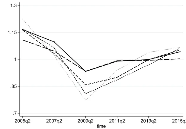
.7 .85 1 1.15 1.3
2005q2 2007q2 2009q2 2011q2 2013q2 2015q2
[image:15.612.151.459.76.289.2]time
Figure 1: House-price indices. The solid line shows average house-price growth imputed from the PSID, the long-dashed line shows median house-price growth imputed from the PSID, the dotted line represents S&P Case-Shiller HPI, the dashed line represents FHFA HPI, and the short-dashed line corresponds to the Zillow index.
the computed house-price growth from the PSID in Table 1 compares reasonably well to the
established HPIs. I compare the imputed house-price growth index from the PSID with the
weighted, repeat-sales HPI based on transactions involving single-family homes, constructed by
the US Federal Housing Finance Agency (FHFA HPI), and with methodologically similar S&P
Case-Shiller HPI. I also use the Zillow Home Value Index (Zillow HVI) for comparison, whose
methodology differs from the two aforementioned HPIs, mainly because it does not rely on repeat
sales. Instead, it utilizes the Z-estimate, an estimated value of a home based on its proprietary
machine-learning algorithm. Zillow’s Z-estimate uses multiple sources of data, including prior
sales, county records, tax assessments, real estate listings, mortgage information, and geographic
information-system data. Importantly, Zillow’s website allows homeowners to view the entire
history of Z-estimates and to report home improvements, which makes the Zillow HVI index
relevant for comparison. The comparative analysis is presented in Figure 1. This figure reports
the average and median house-price growth index imputed from the PSID, S&P Case-Shiller HPI,
During the sample years, the PSID is a biennial survey, in which the overwhelming majority of the
interviews are conducted in the second quarter, which explains the choice of the second quarter
for comparisons. S&P Case-Shiller HPI, FHFA HPI, and Zillow HVI are adjusted accordingly to
show house-price growth for the second quarter of the year relative to the same quarter two years
ago. The three well-known HPIs and the one constructed from the PSID paint the same qualitative
picture during the observed period. The imputed house-price growth closely matches the level
and the pattern of dynamics in house prices over the observed period. The lower volatility of the
imputed house-price growth compared to the S&P Case-Shiller HPI, FHFA HPI, and Zillow HVI
is consistent with the findings in Davis and Quintin (2017) that, whereby, on average, homeowners
tend to report accurate estimates of the current value of their home, during the boom and the bust,
households update the assessments of their homes gradually, such that self-assessed house prices
do not decline as severely as house-price indexes during the bust.
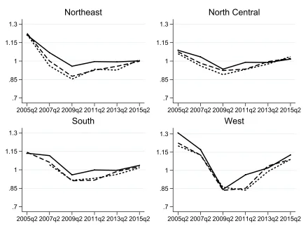
Further analysis shows that similarities between indices’ values are even stronger on a regional
level. The PSID provides information about a state of residence, which I use in constructing a state
and regional measure of the house-price growth index. I compare the imputed house-price growth
index from the PSID to HPIs, available on a state level – FHFA HPI and Zillow HVI. Figure 2
shows the HPIs imputed from the PSID housing data, and the HPI’s by the US Federal Housing
Finance Agency and Zillow over four major regions: Northeast, North Central, South, and West
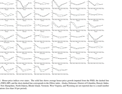
(see Appendix B for the state composition of these regions). State comparisons can be found in
Appendix B, Figure B1. Overall, the house-price growth index, computed from equation (8), is
remarkably close to the HPIs reported by Zillow and the US Federal Housing Finance Agency.
4
Estimation and empirical findings
When consumption and re-investment in housing are simultaneous choices, the choice to reinvest
in housing stock may be directly affected by the consumption choice and correlated with the
.7 .85 1 1.15 1.3
2005q2 2007q2 2009q2 2011q2 2013q2 2015q2
Northeast
.7 .85 1 1.15 1.3
2005q2 2007q2 2009q2 2011q2 2013q2 2015q2
North Central
.7 .85 1 1.15 1.3
2005q2 2007q2 2009q2 2011q2 2013q2 2015q2
South
.7 .85 1 1.15 1.3
2005q2 2007q2 2009q2 2011q2 2013q2 2015q2
[image:17.612.90.530.68.390.2]West
Figure 2: House-price indices over four regions. The solid line shows average house-price growth imputed from the PSID, the dashed line represents FHFA HPI, and the short-dashed line corresponds to the Zillow index.
simultaneous decision-making, and ordinary least-squares estimation of equation (5) could result
in biased estimates. The remedy is to find instruments, such that they are not affected by nondurable
consumption but are correlated with changes in housing stock and use an IV estimation technique
for obtaining consistent estimates of the parameters in equation (5).
As argued in Harding, Rosenthal, and Sirmans (2007), home attributes tend to be correlated
with maintenance and therefore with the changes in housing stock. Indeed, in my data sample,
the correlation between house size and level of maintenance expenditures is positive, significantly
different from zero at the 1% significance level, and equal to 0.13. Also, home attributes have no
natural role in the consumption-model specification (5). Even if home attributes could have affected
time and therefore drop out of the model in first differences. Hence, the observed attributes of a
home, such as house size, can be used as instruments for reinvestment in equation (5).
When households derive utility from consumption and housing, a household’s optimization
problem can be supplemented by one more restriction, namely, the one describing the optimal
choice of reinvestment in housing stock. The resulting demand for housing stock, along with
its dependance on consumption, also depends on house prices (see equation (A4) in Appendix
A). Homeowners actively manage the quantity and quality of their housing stock by implementing
housing improvements, taking prices as given exogenously. House prices have no natural role in the
consumption model (see equations (A3)-(A4) in Appendix A), and being exogenous to nondurable
consumption choice, house prices are relevant for explaining changes in housing stock, making an
excellent instrument. Changes in housing stock and house-price indices (both the imputed
indi-vidual house-price index and the state-level FHFA HPI) are negatively correlated. For example,
the correlation between changes in housing stock and the imputed individual house-price index in
locality is -0.20 and significantly different from zero at the 1% significance level. The negative
correlation between housing stock and house prices is in agreement with the restrictions of the
demand theory, whereby home improvements are expected to react negatively to the increase in
prices. See early empirical estimates of price elasticity of the demand for housing consumption in
Rosen (1979), Hanushek and Quigley (1980), MacRae and Turner (1981), Goodman and Kawai
(1986), and more recently in Goodman (2002) and Ioannides and Zabel (2003). Thus, the
in-struments include house size, the lagged imputed house-price index, which measures house prices
specific to the locality of residence, and the locality-specific house-price index interacted with the
state-of-residence house-price index.
To capture the utility taste shifter, in estimation of equation (5) I include a set of demographic
variables, such as the level of education, change in age squared, and change in family size. Following
Mazzocco (2007) and Meghir and Weber (1996), I also include conditioning variables of the change
in a dummy if the husband works and the change in a similar dummy for the wife, to capture a
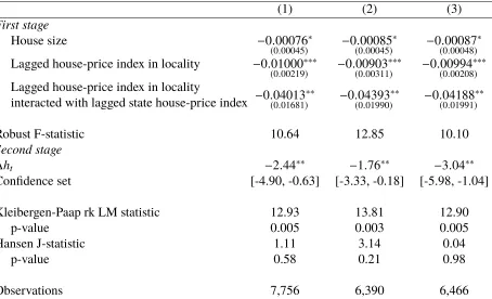
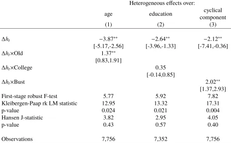
Table 2: Estimation results
(1) (2) (3)
First stage
House size −0.00076∗
(0.00045) −0.00085 ∗
(0.00045) −0.00087 ∗ (0.00048)
Lagged house-price index in locality −0.01000∗∗∗
(0.00219) −0.00903 ∗∗∗
(0.00311) −0.00994 ∗∗∗ (0.00208)
Lagged house-price index in locality
interacted with lagged state house-price index −0.04013
∗∗
(0.01681) −0.04393 ∗∗
(0.01990) −0.04188 ∗∗ (0.01991)
Robust F-statistic 10.64 12.85 10.10
Second stage
∆ht −2.44∗∗ −1.76∗∗ −3.04∗∗
Confidence set [-4.90, -0.63] [-3.33, -0.18] [-5.98, -1.04]
Kleibergen-Paap rk LM statistic 12.93 13.81 12.90
p-value 0.005 0.003 0.005
Hansen J-statistic 1.11 3.14 0.04
p-value 0.58 0.21 0.98
Observations 7,756 6,390 6,466
NOTE: The first-stage results report coefficients; their standard errors are reported in parentheses, clustered by state level, and the Kleibergen-Paap Waldr k F-statistic, adjusted for clustering by state level. Significance levels: 1%***, 5% **, 10% *. The second-stage results report the CUE point coefficient estimates for the change in housing stock. Weak-instrument-robust confidence sets in square brackets are based on a linear combination (LC) test of 5%KandAR
statistics. I also report the Kleibergen-Paapr k LM test of underidentification and Hansen’s J-test of overidentifying
restrictions. Instruments include house size, lagged local house-price index computed as in equation (8), and lagged local house-price index interacted with the lagged state house-price index. All regressions include year dummies, change in a dummy if the husband works, change in a similar dummy for the wife, and demographic controls, such as changes in family size, a householder’s age interacted with education, and age squared.
of leisure that is not formally modelled in this paper. Year dummies are used to capture aggregate
macroeconomic and financial shifters.
Table 2 reports the estimation results for homeowners (column(1)), homeowners with positive
liquidity (column (2)), and homeowners with a low DSR (column (3)). The results from a first-stage
regression of changes in housing stock, reported in Table 2, confirm a negative relationship between
house prices and housing stock. According to the first-stage results, the estimated coefficients on
lagged house-price change in locality and the same interacted with the lagged house-price index
in the state of residence are negative and statistically significant at the 5% significance level. The
correlation between house size and growth in housing stock, the results in Table 2 suggest that after
controlling for the house-price dynamics, smaller homes experience faster growth in housing stock.
Provided that larger homes spend more on repairs and renovation and, per the American Housing
Survey of the US Census Bureau, on average, maintain more adequate home quality than smaller
homes, their housing stock may not grow as fast.
The robust F-statistics for the test of the hypothesis that the coefficients on the excluded
instruments are zero, reported in Table 2, are between 10.1 and 12.9, which is arguably just
outside of the problematic range (Staiger and Stock 1997; Stock and Yogo 2005). Nevertheless,
the moderate values of the F-statistics in Table 2 can suggest the instruments may potentially be
weak. In recognition of this problem, in addition to the robust F-statistics, for each estimation,
I report the robust-to-clustering Kleibergen-Paapr k LM test of underidentification and Hansen’s J-test of overidentifying restrictions. The main parameter of interest is estimated with the GMM continuously updated estimator (CUE), following the evidence in Hahn, Hausman, and Kuersteiner
(2004) that the CUE estimator is more robust to the presence of weak instruments, and in that case,
performs better than the IV or two-step GMM estimators. For all estimations, the Kleibergen–Paap
underidentification LM test rejects the null hypotheses at the 95% level, suggesting the instruments
are adequate to identify the equation. Furthermore, Hansen’sJ-statistic is far from rejection of the
null that the overidentifying restrictions are valid, providing me with confidence that the instrument
set is appropriate. Finally, for the estimated parameter of interest, I report a weak-instrument-robust
confidence set, developed by Andrews (2016). The confidence set is based on a linear combination
(LC) test of K-statistic (a score statistic based on the continuously updating GMM objective function as in Kleibergen 2005) and S-statistic that is a Lagrange multiplier version of the Anderson–Rubin
(AR) weak-instruments-robust test (Stock and Wright 2000).
The presentation of the estimation results keeps the focus on the coefficient on housing-stock
growth ∆ht, which indicates whether an intratemporal dependence exists between nondurable
consumption and housing stock. First, I test whether an intratemporal dependence exists between
by∆htis negative and statistically significant for all samples of homeowners. Overall, the estimation
results reject separability in preferences over nondurable consumption and housing.
Further, the negative sign of the estimated coefficient provides information about the sign of the
mixed partial derivative of the utility function and indicates an increase in housing stock decreases
the marginal utility of nondurable consumption. In the context of power intertemporal utility
combined with the CES intratemporal utility, the negative sign on the mixed partial derivativeUCH
indicates intertemporal consumption smoothing is more important than intratemporal smoothing
(ε > σ in equation (6)). This result agrees with empirical findings on the joint estimation of the
parameters of intratemporal and intertemporal elasticity of substitution (Li et al. 2016; Ogaki and
Reinhart 1998; Yogo 2006). It supports parameterizations of preferences in the life-cycle housing
literature (e.g., the influential studies of Cocco 2005; Yao and Zhang 2005) and financial literature
(Piazzesi, Schneider, and Tuzel 2007).8
Because the results for the full sample of homeowners and the restricted subsamples in columns
(2)-(3) of Table 2 do not differ substantially, the following set of estimations is conducted on the
full sample of homeowners. I test whether an intratemporal dependence exists between separate
categories of nondurable consumption and housing stock. This test is possible under the assumption
that in the utility, distinct categories of consumption are additively separable but may be pairwise
dependent on housing stock. That is, I estimate 10 different models for distinct nondurable
consumption categories and report the findings in Table 3.
The results in Table 3 indicate the coefficient on the change in housing stock in regressions for
most consumption categories is not precisely estimated. Food consumption and consumption of
utility services (gas, heating fuel, electricity, water and sewer, etc.) are notable exceptions. For these
categories of nondurable consumption, the coefficients on the change in housing stock are negative
Table 3: Estimation results for the distinct categories of nondurable consumption
food health education child care clothing recreation transport tel./internet utilities vacations
(1) (2) (3) (4) (5) (6) (7) (8) (9) (10)
∆ht −3.09∗∗ 4.33 -10.67 5.28 -1.96 -2.96 -1.18 -4.45 −2.29∗∗ -1.89
[-6.9,-0.6] [-2.6,13.4] [-31.3,25.9] [-13.1,35.9] [-7.2, 2.1] [-7.4, 1.4] [-6.5, 1.9] [-10.2, 1.7] [-5.3,-0.1] [-10.0,4.3]
First-stage
robust F-test 10.64 12.21 3.79 5.56 9.84 17.56 10.51 10.38 11.04 10.16
rk LM test 12.93 13.24 7.94 8.97 12.07 15.22 12.61 12.74 13.10 13.82
p-value 0.005 0.004 0.047 0.030 0.007 0.002 0.006 0.005 0.004 0.003
J-test 1.05 0.56 0.17 0.05 0.70 2.66 0.96 3.42 0.47 0.02
p-value 0.59 0.76 0.92 0.97 0.70 0.27 0.62 0.18 0.79 0.99
Obs. 7,756 7,360 1,799 853 7,380 6,446 7,587 7,712 7,613 5,359
NOTE: The table reports the CUE point coefficient estimate for the change in housing stock, weak-instrument-robust confidence sets in square brackets based on a linear combination (LC) test of 5%K andARstatistics, the Kleibergen-Paap Waldr kF-statistic, adjusted for clustering by state level, the Kleibergen-Paapr kLM test of underidentification, and Hansen’s J-test of overidentifying restrictions. Significance levels: 5%**, 10% *. Instruments include house size, lagged local house-price index computed as in equation (8), and the lagged local house-price index interacted with the lagged state house-price index. All regressions include year dummies, change in a dummy if the husband works, change in a similar dummy for the wife, and demographic controls, such as changes in family size, a householder’s age interacted with education, and age squared.
and statistically different from zero at the 5% significance level, and the magnitude of the estimated
coefficients is similar to the ones estimated with total nondurable consumption in Table 2. The
finding of nonseparability between housing stock and consumption of utility services is probably not
surprising, because home improvements often target a more efficient usage of water and sewer, gas,
heating fuel, and electricity. Until the relatively recent expansion of the consumption questionnaire,
the PSID survey collected merely the information about food expenditures, which prompted many
authors to use it as a proxy for nondurable consumption. Flavin and Nakagawa (2008) estimate
a model that nests intratemporal nonseparability between nondurable consumption and housing
and a habit-formation component, formulating preferences using the power intertemporal utility
and the CES intratemporal utility and using food-consumption data from the PSID. Unlike the
findings in the literature cited above, and the results reported in this article, Flavin and Nakagawa
(2008) find support for the positive mixed partial derivative of the utility, which, as argued in
their study, in the presence of a transaction cost on housing, is needed for the empirically relevant
limited responsiveness of nondurable consumption to the interest rate. Distinct to this study and the
literature cited above, the assumption on constant housing stock for households who do not move
is a notable feature of the analysis in Flavin and Nakagawa (2008), which can possibly explain the
differences in findings.
Finally, I estimate equation (5), allowing for testing heterogeneous effects in the parameter of
interest over age, education, and cyclical component. To do so, I divide the sample of homeowners
by age group and interact∆ht with a dummy for households older than age 45 (denoted as “Old”
in Table 4). Next, I divide the sample between households with only a high school diploma and
those with a college degree, and interact∆ht with a dummy for households with a college degree
(denoted as “College” in Table 4). Here, I dropped 404 observations for households with less than a
high school education. Lastly, to explore the effect of the cyclical component, I construct a dummy
variable for the period when house prices declined steeply as opposed to periods of prevalently
observed non-declining house prices, and interact∆ht with the bust dummy (denoted as “Bust” in
Table 4: Estimation results for heterogeneous effects over demographic and cyclical components Heterogeneous effects over:
age education cyclical
component
(1) (2) (3)
∆ht −3.87∗∗ −2.64∗∗ −2.12∗∗
[-5.17,-2.56] [-3.96,-1.33] [-7.41,-0.36]
∆ht×Old 1.37∗∗
[0.83,1.91]
∆ht×College 0.35
[-0.14,0.85]
∆ht×Bust 2.02∗∗
[1.37,2.93]
First-stage robust F-test 5.77 5.92 7.82
Kleibergen-Paap rk LM statistic 12.95 13.32 17.31
p-value 0.024 0.021 0.004
Hansen J-statistic 3.82 2.95 4.05
p-value 0.43 0.57 0.40
Observations 7,756 7,352 7,756
NOTE: The table reports the CUE point coefficient estimate for the change in housing stock, weak-instrument-robust confidence sets in square brackets based on a linear combination (LC) test of 5%KandARstatistics, the Kleibergen-Paap Wald rk F-statistic, adjusted for clustering by state level, the Kleibergen-Kleibergen-Paapr kLM test of underidentification, and Hansen’s J-test of overidentifying restrictions. Significance levels: 5%**, 10% *. Instruments include house size, lagged local house-price index computed as in equation (8), and lagged local house-price index interacted with the lagged state house-price index. The instruments are accordingly interacted with the relevant dummies for age, education, and bust. All regressions include year dummies, change in a dummy if the husband works, change in a similar dummy for the wife, and demographic controls, such as changes in family size, a householder’s age interacted with education, and age squared.
The results in Table 4 suggest some heterogeneity is present in the estimates. The nonseparability
between nondurable consumption and housing is largely present for both young and old households,
although it is somewhat weaker for the old households. No decisive heterogeneity is detected
over education groups. The results for the cyclical component reveal possible heterogeneity in
nonseparability over time, and suggest separability between nondurable consumption and housing
may not be rejected during the bust period. This finding, however, is based on only one episode
of declining house prices, observed over the sample period, and calls for a further analysis of the
factors behind it. It can be affected by the relative strength of the intratemporal and intertemporal
of preferences over households’ nondurable consumption and housing stock and by the growth rates
in those consumption goods, which may also maneuver over business cycles.
5
Conclusion
I test for and find evidence of the intratemporal dependence between total nondurable consumption
and housing. My results contribute to the relatively sparse literature investigating the structure
of households’ preferences over durable and nondurable consumption, and the importance of
understanding the preferences over housing and nondurable consumption for academic research and
economic policy warrants further research on this topic. For example, the finding of nonseparability
between nondurable consumption and housing in individual preferences is relevant for testing the
housing wealth effect on consumption. Because I do not rule out intratemporal dependence between
housing and consumption, the tests for other channels between housing prices and consumption
expenditure (wealth effect, collateral channel, common factors) for homeowners may likely be
hindered by the intratemporal tradeoff between housing and consumption. The results may also be
relevant for the life-cycle literature that often relies on preferences over consumption and housing
being additively separable. The evidence on nonseparability in preferences over consumption and
housing, found in this paper, suggests that if economic-policy conclusions strongly rely on the
assumption of additive separability over consumption and housing in an agent’s preferences, then
on the disaggregated level, these conclusions may be sensitive to the composition of the target
group, in particular in relation to households who are long in housing.
References
Aladangady, Aditya.2017. “Housing Wealth and Consumption: Evidence from
Alan, Sule, Orazio Attanasio, and Martin Browning.2009. “Estimating Euler equations with
noisy data: two exact GMM estimators.”Journal of Applied Econometrics24 (2): 309–324.
Andrews, Isaiah. 2016. “Conditional Linear Combination Tests for Weakly Identified Models.”
Econometrica84 (6): 2155–2182.
Attanasio, Orazio P., Laura Blow, Robert Hamilton, and Andrew Leicester. 2009. “Booms
and busts: Consumption, house prices and expectations.”Economica76 (301): 20–50.
Bajari, Patrick, Phoebe Chan, Dirk Krueger, and Daniel Miller.2013. “A dynamic model of
housing demand: Estimation and policy implications.”International Economic Review54 (2): 409–442.
Browning, Martin, Mette Gørtz, and Søren Leth-Petersen. 2013. “Housing Wealth and
Con-sumption: A Micro Panel Study.”The Economic Journal123 (568): 401–428.
Campbell, John Y., and João F. Cocco. 2007. “How do House Prices affect Consumption?
Evidence from Micro Data.”Journal of Monetary Economics54 (3): 591–621.
Carroll, Christopher D., Misuzu Otsuka, and Jiri Slacalek.2011. “How large are housing and
financial wealth effects? A new approach.” Journal of Money, Credit and Banking 43 (1): 55–79.
Case, Karl, John M. Quigley, and Robert Shiller.2005. “Comparing Wealth Effects:The Stock
Market versus the Housing Market.”Advances in Macroeconomics5 (1): 1–34.
Chinloy, Peter. 1979. “The estimation of net depreciation rates on housing.” Journal of Urban Economics6 (4): 432–443.
Cocco, João F. 2005. “Portfolio Choice in the Presence of Housing.” The Review of Financial Studies18 (2): 535–567.
Cooper, Daniel.2013. “House price fluctuations: the role of housing wealth as borrowing
Davis, Morris A., and François Ortalo-Magnè.2011. “Household expenditures, wages, rents.”
Review of Economic Dynamics14 (2): 248–261.
Davis, Morris A., and Erwan Quintin. 2017. “On the Nature of Self-Assessed House Prices.”
Real Estate Economics45 (3): 628–649.
DeFusco, Anthony A.2017. “Homeowner Borrowing and Housing Collateral: New Evidence from
Expiring Price Controls.”The Journal of Finance73 (2): 523–573.
Domeij, David, and Martin Flodèn.2006. “The labor-supply elasticity and borrowing constraints:
Why estimates are biased.”Review of Economic Dynamics9 (2): 242–262.
Epstein, Larry G., and Stanley E. Zin. 1989. “Substitution, Risk Aversion, and the Temporal
Behavior of Consumption and Asset Returns: A Theoretical Framework.” Econometrica 57 (4): 937–969.
. 1991. “Substitution, Risk Aversion, and the Temporal Behavior of Consumption and Asset
Returns: An Empirical Analysis.”Journal of Political Economy99 (2): 263–286.
Fischer, Marcel, and Natalia Khorunzhina.2019. “Housing Decision with Divorce Risk.” Inter-national Economic Review60 (3).
Flavin, Marjorie, and Shinobu Nakagawa. 2008. “A Model of Housing in the Presence of
Adjustment Costs: A Structural Interpretation of Habit Persistence.” American Economic Review98 (1): 474–95.
Gan, Jie. 2010. “Housing Wealth and Consumption Growth: Evidence from a Large Panel of
Households.”Review of Financial Studies23 (6): 2229–2267.
Gayle, Wayne-Roy, and Natalia Khorunzhina.2018. “Micro-Level Estimation of Optimal
Con-sumption Choice With Intertemporal Nonseparability in Preferences and Measurement Errors.”
Goodman, Allen C.2002. “Estimating Equilibrium Housing Demand for “Stayers”.”Journal of Urban Economics51 (1): 1–24.
Goodman, Allen C., and Masahiro Kawai.1986. “Functional form, sample selection, and housing
demand.”Journal of Urban Economics20 (2): 155–167.
Gyourko, Joseph, and Joseph Tracy. 2006. “Using Home Maintenance and Repairs to Smooth
Variable Earnings.”Review of Economics and Statistics88 (4): 736–747.
Hahn, Jinyong, Jerry Hausman, and Guido Kuersteiner.2004. “Estimation with weak
instru-ments: Accuracy of higher-order bias and MSE approximations.”The Econometrics Journal 7 (1): 272–306.
Hanushek, Eric A, and John M Quigley.1980. “What Is the Price Elasticity of Housing Demand?”
The Review of Economics and Statistics62 (3): 449–54.
Harding, John P., Stuart S. Rosenthal, and C.F. Sirmans. 2007. “Depreciation of housing
capital, maintenance, and house price inflation: Estimates from a repeat sales model.”Journal of Urban Economics61 (2): 193–217.
Hicks, John R., and Roy G. D. Allen.1934. “A Reconsideration of the Theory of Value. Part I.”
Economica1 (1): 52–76.
Ioannides, Yannis M., and Jeffrey E. Zabel.2003. “Neighbourhood effects and housing demand.”
Journal of Applied Econometrics18 (5): 563–584.
Jappelli, Tullio.1990. “Who is Credit Constrained in the U. S. Economy?”The Quarterly Journal of Economics105 (1): 219–234.
Jappelli, Tullio, Jörn-Steffen Pischke, and Nicholas S. Souleles. 1998. “Testing for Liquidity
Johnson, Kathleen W., and Geng Li.2010. “The Debt-Payment-to-Income Ratio as an Indicator
of Borrowing Constraints: Evidence from Two Household Surveys.”Journal of Money, Credit and Banking42 (7): 1373–1390.
Kannai, Yakar.1980. “The ALEP definition of complementarity and least concave utility
func-tions.”Journal of Economic Theory22 (1): 115–117.
Kleibergen, Frank.2005. “Testing Parameters in GMM Without Assuming that They Are
Identi-fied.”Econometrica73 (4): 1103–1123.
Li, Wenli, Haiyong Liu, Fang Yang, and Rui Yao. 2016. “Housing over time and over the life
cycle: a structural estimation.”International Economic Review57 (4): 1237–1260.
MacRae, C. Duncan, and Margery Austin Turner.1981. “Estimating demand for owner-occupied
housing subject to the income tax.”Journal of Urban Economics10 (3): 338–356.
Mazzocco, Maurizio.2007. “Household Intertemporal Behaviour: A Collective Characterization
and a Test of Commitment.”The Review of Economic Studies74 (3): 857–895.
Meghir, Costas, and Guglielmo Weber. 1996. “Intertemporal Nonseparability or Borrowing
Restrictions? A Disaggregate Analysis using a U.S. Consumption Panel.” Econometrica 64 (5): 1151–1181.
Mian, Atif, Kamalesh Rao, and Amir Sufi.2013. “Household Balance Sheets, Consumption, and
the Economic Slump.”The Quarterly Journal of Economics128 (4): 1687–1726.
Mian, Atif, and Amir Sufi.2014. House Price Gains and US Household Spending from 2002 to 2006.NBER Working Paper 20152.
Ogaki, Masao, and Carmen M. Reinhart. 1998. “Measuring Intertemporal Substitution: The
Role of Durable Goods.”Journal of Political Economy106 (5): 1078–1098.
Paiella, Monica, and Luigi Pistaferri.2017. “Decomposing the Wealth Effect on Consumption.”
Pelletier, Denis, and Cengiz Tunç. Forthcoming. “Endogenous Life-Cycle Housing Investment
and Portfolio Allocation.”Journal of Money, Credit and Banking.
Piazzesi, Monika, Martin Schneider, and Selale Tuzel.2007. “Housing, consumption and asset
pricing.”Journal of Financial Economics83 (3): 531–569.
Rosen, Harvey S. 1979. “Owner occupied housing and the federal income tax: Estimates and
simulations.”Journal of Urban Economics6 (2): 247–266.
Runkle, David E. 1991. “Liquidity constraints and the permanent-income hypothesis: Evidence
from panel data.”Journal of Monetary Economics27 (1): 73–98.
Samuelson, Paul A.1974. “Complementarity: An Essay on The 40th Anniversary of the
Hicks-Allen Revolution in Demand Theory.”Journal of Economic Literature12 (4): 1255–1289.
Staiger, Douglas, and James H. Stock. 1997. “Instrumental Variables Regression with Weak
Instruments.”Econometrica65 (3): 557–586.
Stock, James H., and Jonathan H. Wright.2000. “GMM with Weak Identification.”Econometrica 68 (5): 1055–1096.
Stock, James, and Motohiro Yogo.2005. “Testing for Weak Instruments in Linear IV Regression.”
InIdentification and Inference for Econometric Models,edited by Donald W.K. Andrews. New York: Cambridge University Press.
Yao, Rui, and Harold H. Zhang.2005. “Optimal Consumption and Portfolio Choices with Risky
Housing and Borrowing Constraints.”Review of Financial Studies18 (1): 197–239.
Yogo, Motohiro. 2006. “A Consumption-Based Explanation of Expected Stock Returns.” The Journal of Finance61 (2): 539–580.
Zeldes, Stephen P. 1989. “Consumption and Liquidity Constraints: An Empirical Investigation.”
Appendix
A
Log-linearized Euler equations
Denote ¯C and ¯H as the expected values of nondurable consumption and housing stock. Let ˆ
C=ln(C/C¯)and ˆH=ln(H/H¯). The subsequent derivations closely follow Mazzocco (2007). Letφ1andφ2be defined as follows:
φ1(Cˆ,Hˆ)=ln
UC(exp{Cˆ}E[C],exp{Hˆ}E[H] ,
φ2(Cˆ,Hˆ)=lnUH(exp{Cˆ}E[C],exp{Hˆ}E[H] ,
where UC and UH are household marginal utilities with respect to consumption and housing.
Assume marginal utilitiesUCandUHare continuously differentiable. Let the one-variable functions
ϑ1 :I1→R and ϑ2: I2 →R be defined as ϑ1(k)= φ1(kCˆ,kHˆ) and ϑ2(k)=φ2(kCˆ,kHˆ), where
I1=(−a,a)andI2=(−b,b). Applying the one-variable Taylor expansion formula with remainder, I get
ϑi(k)=ϑi(0)+ϑ
′
i(0)k+ri(k) for i=1,2 (A1)
with
ri(k)= ∫ k
0
(k−t)ϑi′′(t)dt.
From (A1) and the definition ofϑi(k)withk=1, I get
φi(Cˆ,Hˆ)=φi(0)+
∂φi(0)
∂Cˆ
ˆ
C+∂φi(0)
∂Hˆ
ˆ
H+Ri(Cˆ,Hˆ) for i=1,2. (A2)
Under the assumption of rational expectations, the households’ Euler equations can be written as
βRt+1
UC(Ct+1,Ht+1)
UC(Ct,Ht)
exp(φ′∆zt+1)=1+eCt+1,
βRt+1
Pt
Pt+1
UH(Ct+1,Ht+1)
UH(Ct,Ht)
whereeC
t+1ande
H
t+1are the expectation errors. Taking logs, usingφ1=lnUCandφ2=lnUH, I have
φ1(Cˆt+1,Hˆt+1) −φ1(Cˆt,Hˆt)=−lnβ−lnRt+1−φ∆zt+1+ln(1+eCt+1),
φ2(Cˆt+1,Hˆt+1) −φ2(Cˆt,Hˆt)=−lnβ−lnRt+1−φ∆zt+1+ln(Pt+1/Pt)+ln(1+e H t+1).
By definition of φi(Cˆ,Hˆ), I have ∂φ1/∂Cˆ =UCC/UC, ∂φ1/∂Hˆ =UCH/UC, ∂φ2/∂Cˆ =UHC/UH,
and∂φ2/∂Hˆ =UH H/UH. Then from (A2), UCC
UC ln
Ct+1
Ct +
UC H
UC ln
Ht+1
Ht = −lnβ−lnRt+1−φ∆zt+1−∆R1+ln(1+e
C
t+1), (A3)
UH C
UH ln
Ct+1
Ct +
UH H
UH ln
Ht+1
Ht = −lnβ−lnRt+1+ln
Pt+1
Pt −φ∆zt+1−∆R2
+ln(1+eHt+1), (A4)
where∆Rifori=1,2 is the Taylor-series remainder. Equation (5) follows from rearranging equation
(A3) and writing the resulting equation one period back.
B
Data Construction
B.1
Deflating
Consumption categories reported in the PSID include food, clothing, transportation, utilities, trips
and vacations, entertainment, healthcare, education, and childcare. Deflating of the consumption
expenditures and housing data is closely related to the timing of the relevant survey question. Some
questions ask about expenditures in the month when the interview occurred, whereas others are
asked about the previous year.
Food. Food-consumption expenditures include food consumed at home, away from home, delivered food, and the value of food stamps. Data on food consumed at home and the value of food stamps
are deflated using the CPI for food at home. Data on food consumed away from home and delivered
Table B1: Summary Statistics
2005 2007 2009 2011 2013 2015
Consumption 37,054.3 37,846.0 35,578.4 34,422.7 34,405.9 36,739.3
Food 8,533.6 8,664.8 7,896.8 7,990.7 8,165.7 7,969.0
Clothing 2,112.3 2,079.7 1,790.0 1,819.3 1,599.5 1,700.6
Entertainment 1,173.7 1,232.7 1,247.1 1,127.7 1,108.3 1,084.1 Telecommunications 2,043.5 2,349.1 2,645.0 2,764.6 3,037.3 3,297.5
Utilities 3,269.4 2,933.2 3,070.5 3,145.9 2,937.9 2,953.2
Trips, vacations 2,231.9 2,565.7 2,492.4 2,530.8 2,537.7 2,598.7 Transportation 9,949.9 10,069.4 9,040.8 8,111.2 8,292.3 10,810.9
Education 3,103.0 3,047.0 2,569.7 2,382.7 2,321.0 2,224.8
Childcare 661.9 595.1 686.7 637.5 631.3 478.9
Healthcare 3,975.2 4,309.3 4,139.4 3,912.4 3,775.0 3,621.5
House value 276,241.4 288,350.0 247,357.0 237,246.5 224,979.6 214,371.1
Maintenance 2,795.1 2,926.6 2,460.9 2,427.5 2,217.8 2,271.2
Home size 7.1 7.1 7.0 6.9 6.9 6.8
Age 46.3 48.3 48.3 48.9 49.3 49.6
Years of education 13.8 13.8 14.0 14.1 14.2 14.1
Family size 3.1 3.0 3.0 3.0 3.0 2.9
Household income 85,290.1 87,429.6 88,311.7 81,594.4 84,767.6 85,496.4 Debt service 20,179.4 19,505.2 18,947.5 21,158.6 17,123.7 18,386.8 Fin. liquidity 90,938.0 112,030.2 106,437.9 90,180.4 84,915.2 94,926.1
N homeowners 1,261 1,261 1,556 1,625 1,696 1,618
N with pos.liquidity 1,039 1,039 1,316 1,328 1,390 1,317
N with low DSR 1,053 1,053 1,297 1,357 1,432 1,327
NOTE: All monetary values are in 2009 dollars. For periods 2007 - 2015, the total number of observations for the sample of homeowners is 7,756, for the sample of homeowners with positive financial liquidity is 6,390, and for the sample of homeowners with a low debt-service ratio (DSR) is 6,466.
deflated according to the month and year when the interview occurred, whereas data on food stamps
and income are deflated using the CPI for the end of the year before the interview was conducted.
Clothing. Spending on clothing and apparel is deflated using CPI for apparel for the end of the year before the interview was conducted.
Utility. Utility data include payments for gas or other types of heating fuel, electricity expenses, payments for water and sewer, and other utilities. Each of these utility spending categories is
sewerage maintenance) according to the month and year when the interview occurred.
Communication. Data on telecommunication include payments for telephone, cable or satellite TV, and internet service. Telecommunication data are deflated using CPI for communication according
to the month and year when the interview occurred.
Healthcare. Healthcare spending includes payments for health insurance, prescriptions, in-home medical care and special facilities, doctors, outpatient surgery, dental bills, hospital bills, and
nursing homes. At the time of the interview, the PSID collects healthcare expenditures combined
over two previous years. The total healthcare expenditures are divided by 2 to obtain the value at
the annual frequency, comparable with other expenditure categories. Total spending on healthcare
is deflated using CPI for medical care for the end of the year before the interview was conducted.
Education and childcare. School-related expenses are deflated using CPI for education, whereas childcare expenditures are deflated using CPI for childcare and nursery school for the end of the
year before the interview was conducted.
Entertainment and vacations. Recreation and entertainment spending and expenditures on vacations and trips are deflated using CPI for recreation. Vacations and trips data are deflated according to
the month and year when the interview occurred, whereas recreation and entertainment data are
deflated using the CPI for the end of the year before the interview was conducted.
Transportation. Transportation expenditures are deflated using CPI for transportation. Many of the transportation categories (expenses on gasoline, parking, bus and train, cab fare, vehicle repair,
additional car or lease payments, and other transportation-related spending) are reported for the
month before the interview was conducted and are deflated according to the previous month of the
current year when the interview occurred.
Housing. Housing-related data (home repairs and maintenance, and house value) are deflated using CPI for owners’ equivalent rent of primary residence. House-value data are deflated according to
the month and year when the interview occurred, whereas data on home repairs and maintenance
B.2
US Regions
Figure 2 reports comparisons of the imputed house-price growth from the PSID and the HPIs by
the US Federal Housing Finance Agency and Zillow over four major US regions: Northeast, North
Central, South, and West. Following the regional assignment of the states in the PSID, states were
grouped into regions as follows:
1. Northeast: Connecticut, Maine, Massachusetts, New Hampshire, New Jersey, New York,
Pennsylvania, Rhode Island, Vermont
2. North Central: Illinois, Indiana, Iowa, Kansas, Michigan, Minnesota, Missouri, Nebraska,
North Dakota, Ohio, South Dakota, Wisconsin
3. South: Alabama, Arkansas, Delaware, Florida, Georgia, Kentucky, Louisiana, Maryland,
Mississippi, North Carolina, Oklahoma, South Carolina, Tennessee, Texas, Virginia,
Wash-ington DC, West Virginia
4. West: Arizona, California, Colorado, Idaho, Montana, Nevada, New Mexico, Oregon, Utah,
Washington, Wyoming
The price-growth indices for the fifth region, which includes Alaska and Hawaii, are not reported