Munich Personal RePEc Archive
Age matters
Guo, Danqiao and Boyle, Phelim and Weng, Chengguo and
Wirjanto, Tony
University of Waterloo, Wilfrid Laurier University, University of
Waterloo, University of Waterloo
1 May 2019
Online at
https://mpra.ub.uni-muenchen.de/93653/
Age Matters
Danqiao Guoa, Phelim Boylea,b, Chengguo Wenga, Tony Wirjantoa,c
a
Department of Statistics and Actuarial Science, University of Waterloo
b
Lazaridis School of Business and Economics, Wilfrid Laurier University
c
School of Accounting and Finance, University of Waterloo
Abstract
This paper starts from examining the performance of equally weighted 1/N stock portfolios over time. During the last four decades these portfolios outperformed the market. The construction of these portfolios implies that their constituent stocks are in general older than those in the market as a whole. We show that the differential performance can be explained by the relation between stock returns and stock age. We document a significant relation between age and returns. Since 1977 stock returns have been an increasing function of age apart from the oldest ages. For this period the age effect completely dominates the size effect.
Keywords: Bootstrapped portfolio, rebalanced portfolio, age effect, size effect JEL Classification: G10, G11
1. Introduction
Financial economists have long been interested in the empirical distribution of individual stock
returns. These returns provide the raw inputs for the evaluation of portfolio strategies as well as a
testing ground for asset pricing theories. Indeed Markowitz (1952) in his classic paper on portfolio
selection advocated the use of the empirical distribution of historical stock returns as the first step in
providing parameter estimates for his optimization algorithms. More recently Bessembinder (2018)
has conducted an extensive analysis of individual stocks using returns from the Center for Research
in Securities Prices (CRSP) database.
Portfolios of individual stocks are attractive to risk averse investors because of their potential
diversification benefits. The equally weighted1/N strategy has been widely studied in the finance
Email addresses: [email protected](Danqiao Guo),[email protected](Phelim Boyle),
[email protected](Chengguo Weng),[email protected](Tony Wirjanto)
1
literature. It is a very simple strategy since it involves no estimation, no optimization, no short
positions and has relatively little turnover compared to other strategies. Benartzi and Thaler (2001)
document that it is widely used in practice by participants of defined contribution pension plans as
a heuristic method for choosing asset classes. Despite its naive construction this strategy has been
shown to outperform most alternative strategies. For example DeMiguel et al. (2009) examine the
performance of the 1/N rule using a variety of datasets. They attribute the superior performance
of the equally weighted strategy to the presence of estimation risk and its well known perverse
interaction with optimization.
Brennan and Torous (1999) also demonstrate the superior performance of an equally weighted
1/N rebalanced portfolio over the value weighted market portfolio. They use individual stock
returns from the CRSP database for the period 1926-1997 to construct their equally weighted
portfolio. They attribute this outperformance mainly to the small firm effect:
“because of higher returns on small firms, an equally weighted portfolio of as few as
five randomly chosen firms can provide the same level of expected utility as the value
weighted market portfolio."
Plyakha et al. (2015) show that equally weighted portfolios outperform value weighted portfolio
based on samples of individual stocks in the S&P indices. They show that the major source of the
extra alpha in the equally weighted portfolio is due to the contrarian nature of the strategy.
Our paper examines the performance of equally weighted portfolios and we show that there
is an additional reason for their superior returns. It is worth emphasizing that our portfolios are
made up of individual stocks from the entire CRSP database. In contrast the datasets used by
DeMiguel et al. (2009) where the N components of the equally weighted portfolios are themselves
portfolios1 or indices for seven of their datasets. Their eighth dataset is based on simulated stock
returns for a single factor model. Our equally weighted portfolios are constructed as in Brennan and
Torous (1999). We use the same comprehensive dataset as Bessembinder (2018) since it facilitates
comparisons with his results.
This approach, where the components of the equally weighted portfolios are individual securities
1
rather than other portfolios, is better suited to our purpose. It permits us to keep track of the time
series properties of the individual stocks and in particular their ages. Another difference between
using individual stocks and portfolios is that when a stock is delisted it disappears from the equally
weighted portfolio. If this happens it is replaced with another stock drawn at random from the
available pool. This newly added stock will be representative of the market as a whole in particular
in terms of age. The other stocks in the portfolio will age by one period so that the portfolio as a
whole will grow older.
A simple and effective way to compare the performance of the equally weighted portfolio with
that of the market is to use comparably sized portfolios which contain N equally weighted stocks
at the start of each period. These portfolios are routinely liquidated at the end of each period and
a new set ofN stocks is selected at random from the available pool. By means of this construction
these portfolios are representative of the market as a whole. Bessembinder (2018) used the same
type of construction except that his portfolios were value weighted instead of equally weighted.
Following his convention we refer to these portfolios as equally weighted bootstrapped portfolios
or just bootstrapped portfolios. We denote the traditional 1/N portfolios as equally weighted
rebalanced portfolios or just rebalanced portfolios. One important property of the bootstrapped
portfolios is that because of the periodic rebalancing they have the same2 exposure to reversals as
the traditional1/N portfolios.
The current paper compares the returns on the rebalanced portfolio with the returns on the
bootstrapped portfolio over the 1926-2016 period spanned by the CRSP data base. While there is
some secular variation in the relative performance of the two types of portfolio over time, our most
striking finding is that the rebalanced portfolio yields higher realized returns than the bootstrapped
portfolio during the most recent forty-year period: 1977-2016. This finding is robust to the portfolio
size and to the choice of different starting dates and to the investment horizon within this period.
We contend that this difference is not due to the rebalanced portfolio benefitting from reversals
since the bootstrapped portfolio will also benefit to the same extent. During the 1926-1976 period
the returns on the rebalanced portfolio are very similar to the returns on the bootstrapped portfolio
There are two arguments for why one might not expect the rebalanced portfolio to outperform
2
the market. The first has to do with delisting since holding a stock until it disappears from the
market does not seem to be a smart strategy. Actually, the popular belief that being delisted is bad
news is somewhat misleading. This is because a stock can disappear from the market for reasons
other than bankruptcy. For example the most frequent reason for delisting is merger and acquisition,
which often reflects the past success of a company. Even for the stocks that exit from the market due
to unfavorable reasons investors rarely lose all of their investment. The second reason is that our
results appear to run counter to the size3 effect. If on average portfolios of small stocks outperform
portfolios of large stocks and if it is true that older firms in general tend to be larger than younger
firms and if age is positively correlated with firm size, the stocks in the rebalanced portfolios being
older than average will be larger than the stocks in the bootstrapped portfolios. We explain in the
paper why the situation is much more nuanced than this and we disentangle the intertwined effects
of size and age.
In this paper we argue that the reason for the performance difference between the rebalanced
portfolios and the bootstrapped portfolios stems from the relation between stock age and stock
return. The age distribution of the stocks in the bootstrapped portfolio will be very similar to
that of the stock universe whereas the age distribution of the stocks in the rebalanced portfolio will
typically be older than those in the stock universe. Thus the age profile of the N stocks in the
rebalanced portfolio will be older than those of theN stocks in the bootstrapped portfolio. If stock
return is related to age this will impact the relative performance of the two types of portfolios. We
show in the paper that there is a significant positive relation between stock return and stock age
during the period 1977-2016 and that the relation is much weaker4 during the first fifty years from
1926 to 1976.
This positive relation between age and return is consistent with the underperformance of IPO’s
documented by Ritter (1991). He finds that newly listed firms perform worse on average than a
matched sample of older firms during the first five years after listing. Updated tables providing
3
There is considerable evidence that the importance of the size effect has declined in recent years. See Horowitz et al. (2000), Alquist et al. (2018).
4
data on the long run performance of new issues are available from Jay Ritter’s website5. During the
period 1980-2016 IPO firms have underperformed matched (by size) firms by an average of 3.3%
per annum during the first five years. Brennan and Torous (1999) made this connection6 between
the poor returns on new listings and the composition of the equally weighted portfolios.
The relation between firm age and stock return is also consistent with the recent model of Lin
et al. (2018) who analyze the conditions under which firms adopt new technology. In their setup
firms differ in their capacity to adopt new (and costly) technology which will make them more
efficient. The authors define the concept of capital age as the length of time since the last adoption
of a new technology. Capital age is used to measure different levels of technical efficiency. Young
capital age firms are closer to the technological frontier than old capital age firms. Young capital
age firms are predicted to be more productive and less risky than old capital age firms. Hence
they earn lower expected returns than old capital age firms and this is confirmed empirically. Our
measure of calendar age bears a similar relation to expected return.
To better understand the age effect and the connection between the age effect and the size effect
we construct 16 portfolios that are doubly sorted into four age groups and four size groups and
compare their performance. We focus on the 1977-2016 period and report comparable results for
the 1926-1976 period in Appendix A. The age effect is clearly observed in all size groups, and the
size effect is evident in all age groups. When we divide stocks into four age groups we find that
returns are increasing with age over the first three groups but are flat or drop a little for the oldest
group. That is the age effect is not monotone. It holds over the bulk of a firm’s life but may be
reversed in the oldest age group. Hence our age effect is not inconsistent with the finding that firms
are less profitable at older ages (see for instance Loderer and Waelchli (2010)).
This leads us to conclude that the age and size are not spanned by a common underlying factor.
Moreover the age effect seems to be in conflict with the size effect, since stock age and size are
positively correlated but explain the stock returns in the opposite direction. To further resolve
5
https://site.warrington.ufl.edu/ritter/ipo-data/ 6
this puzzle we divide stocks into decile groups based on their age or size and calculate the return
statistics within each decile group. The results suggest that the observed small firm effect is a result
of the extremely positive return skewness in the smallest 10% of the stocks (This has been noted in
Bessembinder (2018), and the general return skewness problem is discussed in Heaton et al. (2017)
for instance). If the within-group median return is used as the performance measure, the direction
of how the two factors affect stock returns turns out to be the same.
This paper makes the following contributions to the literature. First, we acquire deeper
under-standing of why the rebalanced portfolio outperforms the bootstrapped portfolio so impressively
over the period from 1977 to 2016. We show that this is caused by a combination of the older
age profile of the rebalanced portfolio and the relation between stock returns and firm age.
Sec-ond, we empirically document an age effect: an asset pricing anomaly that is entangled with but
quite distinct from the size effect. Third, our results provide a possible opportunity for investment
management. An institution could in principle structure a portfolio to exploit the age effect.
The remaining part of this paper is organized as follows. Section 2 analyzes the performance
of the equally weighted bootstrapped portfolio and the equally weighted rebalanced portfolio and
highlights the performance gap. Section 3 relates the performance gap to the difference in age
distribution between the two portfolios and discusses some aspects of the age effect. We provide
a detailed analysis of the these phenomena for the period 1977-2016 and give a summary of the
results for the first 50 years of data in Appendix A. Section 4 discusses economic explanations for
the age effect. Section 5 concludes the paper.
2. Bootstrapped versus Rebalanced Portfolios
In this section we compare the realized returns on our two basic portfolio strategies. These
are the conventional 1/N equally weighted strategy7 that has been studied by DeMiguel et al.
(2009) and the equally weighted bootstrapped strategy. We use the same data as Bessembinder
(2018). The data is available from the Center for Research in Securities Prices (CRSP) monthly
stock return database. As in Bessembinder (2018) only common stocks with share codes 10, 11,
and 12 are included in the study. The entire period runs from June 1926 to December 2016 and
7
includes 26,051 distinct CRSP permanent numbers (PERMNOs). The monthly returns are inclusive
of reinvested dividends.
We construct the bootstrapped portfolio by picking N stocks at the start of each month and
investing equal amounts in each stock. We hold this portfolio for one month before liquidating
the portfolio and starting this process all over again for the next month. By compounding all the
monthly8returns we obtain the holding period return of the bootstrapped portfolio. The rebalanced
portfolio is constructed by selecting N random stocks at inception and investing equal amounts in
each stock. Each month the weights are adjusted to obtain equal investments in each stock. If a
stock in this portfolio is delisted in a particular month it is replaced by another stock selected at
random from the available pool of actively traded CRSP stocks at that time.
2.1. Relative Performance
We compare the performance of the bootstrapped and rebalancedN-stock portfolios in Table 1
and find that on average the returns on the rebalanced portfolios exceed those on the bootstrapped
portfolios. These results are based on simulations of 20,000 portfolios of each type forN = 5,25,50,
or 100. As noted previously in the Introduction these results may appear counterintuitive. They
provide the motivation for investigation of the age effect in the next section.
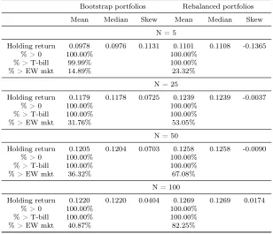
Comparing the mean annualized returns in the same rows, we notice that the rebalanced
port-folios outperform the bootstrapped portport-folios for all four values of N. For N = 5the performance
gap is 1.23% per annum. This pattern becomes even more obvious when we look at the percentage
out of the 20,000 portfolios that outperform the equally weighted portfolio of the whole market. For
the bootstrapped portfolios, as the portfolio size increases, this percentage increases toward 50%9.
However the proportion of rebalanced portfolios that outperform the equally weighted market
grad-ually increases to be over 80%. Note we have not yet taken transaction costs into account when
8
It is worth pointing out that some stocks enter the bootstrapped portfolio in their last trading month and are delisted during the month. These stocks are associated with a code of delisting reason and a delisting return. The delisting return is calculated by comparing the security’s Amount After Delisting with its price on the last day of trading. In such a case we adjust the stock return by incorporating the delisting return to reflect the actual return an investor would obtain when holding the stock till it is delisted. There are a few occasions where the delisting reason is specified but the delisting return is missing. In such occasions we follow the method proposed in Shumway (1997) to fill the delisting return according to the delisting reason .
9
Table 1: Summary of annualized returns of 20,000 bootstrapped and rebalancedN-stock portfolios. In a bootstrapped portfolio the indicated numbers of stocks are selected at random for each month. In a rebalanced portfolio the indicated numbers of stocks are selected at random at the beginning of investment horizon, the same stocks are adjusted to have equal weights each month unless one or more stocks are picked at random to make up for the delisted one(s). Equally weighted portfolio returns are computed each month and are linked over the horizon from July 1926 to December 2016. Annualized return is recorded for each of 20,000 simulations of each portfolio type. Mean, median, and skewness of the 20,000 annualized returns are reported, as well as the percentage out of the 20,000 returns that are positive, greater than the return on Treasury bill, and greater than the return on an equally weighted portfolio of the whole market.
Bootstrap portfolios Rebalanced portfolios
Mean Median Skew Mean Median Skew
N = 5
Holding return 0.0978 0.0976 0.1131 0.1101 0.1108 -0.1365
% > 0 100.00% 100.00%
% > T-bill 99.99% 100.00%
% > EW mkt 14.89% 23.32%
N = 25
Holding return 0.1179 0.1178 0.0725 0.1239 0.1239 -0.0037
% > 0 100.00% 100.00%
% > T-bill 100.00% 100.00%
% > EW mkt 31.76% 53.05%
N = 50
Holding return 0.1205 0.1204 0.0703 0.1258 0.1258 -0.0090
% > 0 100.00% 100.00%
% > T-bill 100.00% 100.00%
% > EW mkt 36.32% 67.08%
N = 100
Holding return 0.1220 0.1220 0.0404 0.1269 0.1269 0.0174
% > 0 100.00% 100.00%
% > T-bill 100.00% 100.00%
calculating the returns. That is, since the rebalanced portfolios have much less turnover compared
[image:10.612.152.462.222.482.2]with the bootstrapped ones, the former will be more favourable if transaction costs were included.
Table 2: Summary of annualized returns of 20,000 bootstrapped and rebalanced 100-stock portfolios over three shorter holding periods: July 1926 - December 1976, January 1977 - December 2016, and January 2007 - December 2016. Construction of bootstrapped and rebalanced portfolios is the same as described in Table 1 except that the monthly returns of equally weighted portfolios are linked over indicated investment horizons and that the portfolio size is fixed atN= 100. Annualized return is recorded for each of 20,000 simulations of each portfolio type. Mean, median, and
skewness of the 20,000 annualized returns are reported, as well as the percentage out of the 20,000 returns that are positive, greater than the return on Treasury bill, and greater than the return on an equally weighted portfolio of the whole market.
July 1926 - December 1976
Bootstrapped portfolios Rebalanced portfolios
Mean Median Skew Mean Median Skew
Holding return 0.1167 0.1167 -0.0058 0.1159 0.1159 -0.0050
% > 0 100.00% 100.00%
% > T-bill 100.00% 100.00%
% > EW mkt 45.01% 35.07%
January 1977 - December 2016
Bootstrapped portfolios Rebalanced portfolios
Mean Median Skew Mean Median Skew
Holding return 0.1286 0.1284 0.0913 0.1518 0.1517 0.0605
% > 0 100.00% 100.00%
% > T-bill 100.00% 100.00%
% > EW mkt 41.36% 99.36%
January 2007 - December 2016
Bootstrapped portfolios Rebalanced portfolios
Mean Median Skew Mean Median Skew
Holding return 0.0579 0.0575 0.1110 0.0728 0.0728 -0.0302
% > 0 99.91% 100.00%
% > T-bill 99.69% 100.00%
% > EW mkt 45.44% 78.28%
While Table 1 demonstrates that the returns on the rebalanced portfolios are consistently higher
than those on the bootstrapped portfolios, the differences for N = 50 and N = 100 do not seem
large at around fifty basis points. However recall that these results are based on the entire 90
year period from 1926 to 2016 and that there were relatively few stocks at the start of this period.
We obtain more interesting and more dramatic results when we divide the period up into smaller
subperiods. We redo the same calculations as in Table 1 but based on shorter investment horizons.
The first period is from July 1926 to December 1976 which leads to a holding period of about 50
years. The second period from January 1977 to December 2016 coincides with a typical time period
that would be currently used for asset pricing empirical tests. The third period is from January
Table 2 reports the performance of the bootstrapped and rebalanced portfolios over these
sub-periods. There is a substantial difference in the relative performance of the two portfolios in the
first fifty years and in the last forty years. During the earlier period the returns are very close with
the bootstrapped portfolio being marginally better by0.08%per annum. However during the most
recent forty years the returns on the rebalanced portfolio are on average 2.32% per annum higher
than those on the bootstrapped portfolio. For the most recent decade (2007-2016) the rebalanced
portfolio return is 1.49% per annum higher than the return on the bootstrapped portfolio. We
recall from Table 1 that over the entire 90 year period withN = 100 that the mean return on the
rebalanced portfolio exceeds the mean return on the bootstrapped portfolio by 0.49% per annum.
This suggests something quite different is happening in the last four decades as compared to the
first five decades.
2.2. How Bad is Being Delisted?
In the Introduction we mentioned that some observers tend to think that the rebalanced portfolio
would perform poorly because it holds a stock until it disappears from the market. However it is
sometimes overlooked that being delisted is not necessarily bad news. We refer readers to Table 2B
in Bessembinder (2018) for a detailed summary of lifetime buy-and-hold returns by final delisting
status. The results suggest that the majority of stocks that are finally delisted due to Merger,
Exchange, or Liquidation yield a lifetime buy-and-hold return exceeding that of the one-month
Treasury bill. Even for the stocks that are delisted by the exchange, the mean lifetime
buy-and-hold return is −0.8%, which is far from a devastating outcome. However it should be noted that
this is thanks to the diversification effect - the median lifetime buy-and-hold return is much more
negative. In addition more stocks were delisted due to Merger, Exchange, or Liquidation than any
other reasons. These results together explain why delisting does not unduly penalize the returns on
the rebalanced portfolios.
2.3. Comparison with Value Weighted Bootstrapped Portfolio
We can gain additional insight by comparing the returns on equally weighted strategies with the
returns on value weighted strategies. Specifically we compare the performance of equally weighted
has already computed the returns on value weighted bootstrapped portfolios and we compared his
results with our equally weighted bootstrapped portfolios. In our comparison we use the same set
of stocks in each comparison pair so that the portfolios differ only by their respective weights. We
find10 that the returns on the equally weighted bootstrapped portfolios are on average 2.24% per
annum higher than the returns on the value weighted bootstrapped portfolios. Since both portfolios
have the same age distribution this performance cannot be explained by an age effect. It is due to
the contrarian nature of the equally weighted portfolio and the small firm effect. As we will see in
the next section the equally weighted rebalanced portfolio and the equally weighted bootstrapped
portfolio have quite different age distributions and this can impact their relative performance.
3. Stock Age and Cross-sectional Returns
In this section we demonstrate that stock age is an important determinant of returns. In
particular we show that portfolio age is a key difference between the bootstrapped portfolios and
the rebalanced ones and that this difference leads to the performance gap between these two portfolio
types. The numerical analysis presented in this section is based on the period 1977-2016. This is
because the recent 40-year period is more relevant to the current financial market. For completeness
we report the corresponding results for the period 1926 to 1976 in Appendix A. The age effect is
observable but much weaker during this earlier period.
3.1. A Probabilistic View on Age Distribution
In this subsection we explain using a probabilistic argument why the rebalanced portfolio will
have an older age distribution than the bootstrapped portfolio. Consider a rebalancing date when
there are M stocks available in the stock universe. Then each of the M stocks has a probability
of N/M of being included in the N-stock bootstrapped portfolio. If K stocks that were in the
rebalanced portfolio in the previous period leave the portfolio because of delisting, then theN−K
stocks that already exist in the rebalanced portfolio will remain in the portfolio with a probability
of one. Moreover each of the remaining M −(N −K) stocks in the pool will be selected into
the rebalanced portfolio with a probability of K/(M −N +K) (<N/M). From this perspective
10
an important difference between the two portfolio types rests squarely on the rebalanced portfolio
favouring seasoned stocks by assigning them a much higher probability of staying in the portfolio. In other words the component stocks in the rebalanced portfolio become mature in terms of age
as time elapses. In contrast, the bootstrapped portfolio does not take into account the age of the
stocks. This means that the average age of the rebalanced portfolio will increase over time, whereas
the average age of the bootstrapped portfolio will be similar to that of the stock universe.
Figure 1 shows the profile of the stock population in the CRSP data from 1977 to 2016. The
red portion in each bar represents the number of stocks that entered the universe in the current
calendar year. The blue portion represents the number of stocks that have existed in the universe
at the beginning of each calendar year. In demographic parlance the new listings correspond to
births and the delistings correspond to deaths. The crude birth rate is the total number of births
in a given year divided by the size of the population. The crude death rate is the total number of
deaths in a given year divided by the size of the population. For this data the average crude birth
rate for the period 1977-2016 is 10% while the crude death rate is 9%. These numbers are similar11
to those obtained by Loderer and Waelchli (2010) but higher12than those obtained by Doidge et al.
(2017) who focus only on domestic US stocks. A delisting rate of 10% implies that in the rebalanced
portfolio about 90% of the constituent stocks remain in place each year and as a result they age by
one year. The other ten percent that are added to the portfolio will have an age distribution similar
to that of the stock universe. The age distribution of the bootstrapped portfolio reflects the age
distribution of the stock universe. Hence the average age of the stocks in the rebalanced portfolio
increases13.
3.2. Age Distribution in Bootstrapped and Rebalanced Portfolios
Before presenting the age distributions for different portfolios, it is useful to clarify the calculation
of age in our study. On any given month the age of a stock is the number of months that have elapsed
since the first month the stock appeared in the CRSP database divided by twelve. Our empirical
11
Based on the period 1978-2004, Loderer and Waelchli (2010) obtained 10.3% for the crude birth rate and 9.9% for the crude death rate.
12
Doidge et al. (2017) estimate an average crude birth rate of 7.5% and an average crude death rate of 8.2% based on the period 1975-2012. They just focus on US stocks whereas we follow Bessembinder (2018) and retain securities with share codes 10, 11 and 12. Hence our rates are higher.
13
Figure 1: Population of stocks in the CRSP database: existing stocks and new listings. The figure shows the change in the stock population in the CRSP database from 1977 to 2016. The red portion in each bar represents the number of stocks that entered the universe in the indicated calendar year. The blue portion represents the number of stocks that have existed in the universe at the beginning of the indicated calendar year.
data confirm our predictions about the difference in age distribution between the bootstrapped
and rebalanced portfolios. We consider the holding period from January 1977 to December 2016
and simulate 1000 bootstrapped portfolios as well as 1000 rebalanced portfolios, each containing
100 component stocks. In each month we record the age of all component stocks in each simulated
portfolio. We report the empirical age distribution in both portfolios over each decade in the 40-year
horizon according to the aggregate result across 1000 simulations. The aim of this decade-by-decade
breakdown is to highlight the evolution of the age distribution in the two portfolios as time passes.
Figure 2 presents the age distribution of the two representative portfolios over time. Furthermore,
based on the 1000 simulations, we report the average age of component stocks in each portfolio type
over the four non-overlapping decades. The result is shown in Table 3.
Some institutional background is helpful in interpreting these graphs. The average age of the
entire stock universe is increasing over these four decades for two main reasons. The first is due to
entry is shown clearly in Figure A.1 of Appendix A. The second is due to the decline14 in new
listings since the mid 1990’s as evidenced by Figure 1. From Figure 2 we see that the histograms
of the age distribution of both the bootstrapped portfolio and the rebalanced portfolio move to the
right over the four decades. However if we compare the histograms of the two portfolios across each
decade we see that the age histogram of the rebalanced portfolio is consistently further to the right
of the corresponding histogram of the bootstrapped portfolio. Table 3 confirms this observation.
The age difference is 4.3 years for the period 1977-1986 and averages 12 years over the next three
decades. The fact that the stock universe is replenished each year with newly listed stocks and the
way in which the rebalanced portfolio is constructed leads to the difference in the age distributions
[image:15.612.78.527.353.592.2]between the two portfolio types.
Figure 2: Age distribution in 100-stock bootstrapped and rebalanced portfolios over different time periods. The distributions are based on age of components of one thousand 100-stock bootstrapped and rebalanced portfolios held over the period from January 1977 to December 2016. We report the empirical age distribution in both portfolios over each decade in the 40-year horizon.
3.3. Age Effect
We have identified the age distribution as a key difference between the bootstrapped and
rebal-anced portfolios. The next step is to investigate whether age can explain the cross-section of stock
14
Table 3: Average age of 100-stock bootstrapped and rebalanced portfolios over different time periods. The average ages are calculated based on age of components of one thousand 100-stock bootstrapped and rebalanced portfolios held over the period from January 1977 to December 2016. We report the average age in both portfolios over each decade in the 40-year horizon.
Portfolio Type 1977 - 1986 1987 - 1996 1997 - 2006 2007 - 2016
Bootstrapped 11.60 11.24 12.90 17.35
Rebalanced 15.90 22.11 25.61 29.89
returns. If age is a significant predictor of stock returns, then the performance gap between the
rebalanced and bootstrapped portfolios can be explained by the difference in the age distributions.
To study the age effect we include each stock that has ever appeared in the stock universe
from January 1977 to December 2016 in our analysis. Each month we record the age and monthly
return (annualized by multiplying by 12) of each stock in the entire universe. Let Rit denote the
annualized return15 of the ith stock in the tth month and Ait denote the age of the ith stock in
the tth month. Now that the data has both time-series and cross-section dimensions, panel data
modeling techniques are used to estimate the parameter of interest, which is the effect of age on
asset returns. Equation (1) is a simple (time effects) model relating the stock’s return to its age16.
Rit =βAit+γt+ǫit (1)
The parameter β quantifies the change in the cross-sectional stock return when the stock age
in-creases by one unit. The parameter γt characterizes the level of average cross-sectional returns in
thetth month. The time effect term is included because the market movement from month to month
could make it problematic to pool samples across time and thus affect the estimation of the age
effect. In addition it can be argued that the age effect in the panel-data regression in equation (1)
is potentially confounded by vintage years. A vintage year is the year in which a company receives
its first influx of investment capital. It is the year when capital is contributed by a venture capital,
a private equity fund or a partnership drawing down from its investors. A vintage year at the
peak or bottom of a business cycle can potentially affect subsequent returns on initial investment
as the company undergoes over or under-valuation at the time. The introduction of the time effect
15
The purpose of annualizing the monthly returns is to bring the estimate of the model coefficient to a more visible scale.
16
in the panel-data regression in equation (1) can be viewed as a rough measure to control for this
potentially omitted confounding influence. Lastly, ǫit is the error term.
Subtracting the cross-sectional average R¯t = N1
t
P
iRit, where Nt is the number of existing stocks in the tth month, from the initial model equation (1) becomes
¨
Rit=βA¨it+ ¨ǫit, (2)
whereR¨it=Rit−R¯t,A¨it=Ait−A¯tand ¨ǫit=ǫit−ǫ¯t. Note thatA¯t and¯ǫtare defined in the same
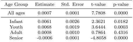
way asR¯t. The first row in Table 4 summarizes the estimation and hypothesis testing results of the
time effects model. The sign of the βˆ and the highly significant p-value for the t-test confirm age
has a significantly positive impact on the cross-sectional return of a stock. In other words, stocks
[image:17.612.192.420.406.479.2]that are older tend to outperform younger stocks.
Table 4: Empirical results for time effects model: January 1977 - December 2016. In the first row, the estimate, standard error, t-statistics, and the associated p-value for the overall time effects model are reported. In each month, the age group each stock belongs to is determined based on the cross-sectional ranking of the stock’s current age. The breakpoints between age groups are the first quartile, median, and third quartile of the cross-sectional age distribution. All stock-month observations are divided into four age groups in this way. In each of the second to fifth rows, model fitting results for the indicated age group are reported.
Age Group Estimate Std. Error t-value p-value
All ages 0.0007 0.0001 7.7808 0.0000
Infant 0.0061 0.0026 2.3621 0.0182 Youth 0.0068 0.0019 3.6444 0.0003 Adult 0.0008 0.0010 0.7864 0.4316 Senior -0.0006 0.0001 -4.8058 0.0000
We fit the same regression model with sub-groups of the data to provide additional robustness to
our result. At the beginning of each month in the investment horizon, each stock in the universe is
labeled with one of the four age groups, Infant, Youth, Adult, and Senior, according to their current
age. The breakpoints between adjacent age groups are the first quartile, median, and third quartile
of the cross-sectional age distribution17. In this way we add an additional categorical feature to each
stock-month observation. Then we divide the data into four sub-groups according to the age group
label and fit the model in equation (1) using each of the four subsets. The estimation and hypothesis
testing results are also presented in Table 4. Within each of the youngest two age groups there is a
17
significant and positive relationship between stock age and stock return. The age-return relation in
the second oldest age group is insignificant. A significant and negative age effect is observed in the
oldest age group which represents a downturn in performance when a stock gets really old. However
the magnitude of the coefficient in the two younger age groups is nine times larger than that in the
two older age groups. The sub-group analysis allows us to acquire a deeper understanding of the
nature of the age effect at different stages of a firm’s life cycle.
We claim that the significant relationship between a stock’s age and its return, together with
the difference in age distribution between the bootstrapped and rebalanced portfolios, explains the
performance gap between these two types of portfolios. We show in Appendix B that the returns
on the rebalanced and bootstrapped portfolios have the same exposure to mean reversion so that
any performance difference cannot be attributed to mean reversion. This does not contradict the
results of Plyakha et al. (2015) which show that the performance of the rebalanced 1/N portfolio
does benefit from mean reversion. The performance of the bootstrapped 1/N portfolio benefits
from mean reversion to the same extent. When we compare returns on the two portfolios, the
impact of mean reversion cancels out so that the difference in returns on the two portfolios cannot
be accounted for by mean reversion.
3.4. Age Effect vs. Size Effect
The small firm effect is a well-known pricing anomaly in finance which holds that smaller firms, or
those companies with a small market capitalization (as a product of price and number of outstanding
shares), outperform larger companies. This effect has been documented by many researchers (see
Van Dijk (2011) for a review) but the consensus is (cf Alquist et al. (2018)) that it has become less
important in more recent years. In results not reported here we confirmed its presence in our data
as well.
In the previous subsection we showed that senior firms generally outperform junior firms. The
“senior firm effect" and the “small firm effect" seem to be complementary (and not substituting)
effects, because a stock’s age and its market capitalization are positively correlated measures of
scale of the issuing company. However these two measures explain the cross-sectional stock returns
in opposite directions since age and size are positively correlated. We confirm the presence of this
current month as well as the ranking (according to age and size respectively) of each stock within
the current stock universe. Pooling the records across months we obtain vectors of stock age, size,
rank by age, as well as rank by size. The correlation coefficient between the raw values of age and
size is 0.23, and the correlation coefficient between the rank of age and rank of size is 0.29.
The finding that two positively correlated stock characteristics explain the cross-sectional stock
returns in opposite directions is puzzling at first. To give a more detailed picture of how the age and
size factors affect stock returns, we construct quartile portfolios which are doubly sorted according
to both the age and size factors. At the beginning of each month all stocks in the universe are
divided into four roughly equal-size age groups, i.e., Infant, Youth, Adult, and Senior, according to
their current age. The breakpoints between adjacent groups are the first quartile, median, and third
quartile of the stock age distribution in the particular month18. Within each of the four age groups,
the stocks are further divided into four size groups, i.e., Tiny, Small, Medium, and Big, according to
their current market capitalization. The doubly sorting procedure yields 16 roughly equal-size stock
groups. For each of the 16 groups we construct an equally weighted portfolio. At the beginning of
each month all these doubly sorted factor portfolios are liquidated and reconstructed to reflect the
change in group members. The portfolio construction date in our study is the beginning of January
1977. All of the portfolios formed on age and size are rebuilt each month until the end of December
2016. Table 5 summarizes three performance measures of these 16 portfolios, namely the annualized
return, the standard deviation, and the Sharpe ratio. The riskless rate used in the calculation of
Sharpe ratios is downloaded from the Kenneth French website19. A comparison among these doubly
sorted quartile portfolios reveals how each factor affects cross-sectional stock returns.
Table 5 displays two main features in the returns. It confirms the existence of both an age
effect and a size effect. We focus initially on the age effect since the size effect is already well
documented in the literature. The age effect is quite pronounced but it is not uniformly monotonic
across all age groups. The average returns generally increase as the age group moves through the
first three age groups. There is a slight decrease in returns as we move from the third age group
to the oldest age group for three of the four size groups. An exception occurs for the third largest
18
This grouping method leads to a dynamic group membership. Size of different groups may be different because there may be multiple stocks at the breakpoint ages.
19
Table 5: Performance of sixteen doubly sorted equally weighted portfolios formed on age and size. Starting from January 1977, at the beginning of each month each available stock is assigned to one of sixteen factor portfolios based on its cross-sectional ranking of age and size. The breakpoints between adjacent age/size groups are the first quartile, median, and third quartile of the age/size distribution. the returns on equally weighted portfolio of all stocks in each factor portfolio are calculated. All factor portfolios are held until December 2016. The average annualized return, standard deviation, and Sharpe ratio of all sixteen portfolios are reported.
Age Group Size Group Return Std Dev Sharpe
Infant
Tiny 13.61% 26.75% 0.34 Small 8.89% 23.52% 0.18 Medium 10.66% 24.80% 0.25 Big 12.66% 23.97% 0.34
Youth
Tiny 17.58% 24.08% 0.54 Small 11.05% 21.21% 0.31 Medium 12.24% 21.21% 0.36 Big 12.17% 20.22% 0.38
Adult
Tiny 21.20% 23.32% 0.71 Small 16.47% 21.32% 0.56 Medium 15.81% 20.27% 0.55 Big 14.23% 17.97% 0.54
Senior
Tiny 20.43% 22.92% 0.69 Small 14.62% 19.62% 0.51 Medium 16.12% 18.80% 0.61 Big 13.79% 15.38% 0.60
size group which we have denoted as the Medium sized group. However we notice that with the
size group fixed, the returns of the two oldest age groups (Adult and Senior) are very close to each
other, and each is much higher than the returns of the two youngest age groups. The closeness in
performance between the oldest two age groups explains why the rebalanced portfolios outperform
the bootstrapped ones notwithstanding the apparent non-monotonicity of the age effect. It is also
worth pointing out that the size factor is not monotone either. Within all of the age groups, the
size group Tiny always outperforms the size group Big, yet the performance does not deteriorate
monotonically with size. The important implication of our findings is that stocks that are both
mature and small tend to outperform the market. These two features, although seemingly having
opposite effects, when appearing together can lead to profitable returns.
The Sharpe ratio results in Table 5 provide an even more striking demonstration of the age
effect. For each size group the Sharpe ratio of the oldest age group is typically double the Sharpe
ratio of the youngest age group. For the first three size groups the Sharpe ratio of the most senior
age group is at least twice the Sharpe ratio of the youngest age group. For the largest size group
the Sharpe ratio of the oldest age group is 1.8 times the Sharpe ratio of the youngest age group.
On the other hand if we hold age fixed the Sharpe ratios of the different size portfolios are much
Table 6: Returns of sixteen doubly sorted equally weighted portfolios: by decade. Starting from January 1977, at the beginning of each month each available stock is assigned to one of sixteen factor portfolios based on its cross-sectional ranking of age and size. The breakpoints between adjacent age/size groups are the first quartile, median, and third quartile of the age/size distribution. The average return on an equally weighted portfolio of all stocks in each factor portfolio is calculated. All factor portfolios are held until December 2016. Annualized returns over the four non-overlapping decades of each factor portfolio are reported.
January 1977 - December 1986 January 1987 - December 1996
Tiny Small Medium Big Tiny Small Medium Big
Infant 23.40% 17.71% 16.86% 17.64% Infant 11.68% 4.22% 10.59% 16.50% Youth 22.38% 13.66% 14.52% 14.35% Youth 21.38% 7.79% 10.96% 13.54% Adult 26.00% 25.84% 22.95% 30.12% Adult 26.17% 11.04% 12.29% 15.64% Senior 30.12% 21.80% 22.31% 17.23% Senior 20.72% 10.35% 13.50% 14.94%
January 1997 - December 2006 January 2007 - December 2016
Tiny Small Medium Big Tiny Small Medium Big
Infant 18.70% 10.13% 8.70% 8.90% Infant 0.65% 3.48% 6.49% 7.61% Youth 21.88% 15.75% 14.89% 11.47% Youth 4.68% 7.00% 8.58% 9.30% Adult 23.56% 18.92% 16.35% 12.52% Adult 9.08% 10.09% 11.65% 9.11% Senior 20.41% 15.14% 17.01% 13.32% Senior 10.45% 11.16% 11.65% 9.67%
Since the age effect is the key finding in our paper, we explore its robustness across different
periods. Table 6 contains a more detailed decade-by-decade breakdown of the doubly sorted
port-folios. This breakdown shows clearly that the age effect is both strong and persistent across all four
decades. For all decades the returns are generally increasing in age. The age group Youth has in
general higher returns than age group Infant with the average difference being 1.80% over all size
groups and decades. In turn age group Adult has in general higher returns than age group Youth
with the average difference being 4.33% over all size groups and decades. Age groups Adult and
Se-nior represent the two oldest groups. The difference between the two oldest age groups is somewhat
lower and negative. Over all the 16 combinations, the average return for age group Senior is lower
than the average return for age group Adult. The average difference is 1.35% per annum which is
small relative to the other differences. These results are consistent with our earlier regression results
in Table 4.
We obtain a more compelling demonstration of the impact of age when we combine the two
youngest age groups by taking their average and the two oldest age groups in the same way. The
group containing the two youngest age groups is labelled Junior and the group containing the two
oldest age groups is labelled Senior. The left hand side of Table 7 compares the returns on these
age sorted portfolios over four size groups for each of the four decades. Differences between the
Table 7: Analysis of portfolios formed on age and size: for each decade. The sixteen factor portfolios are re-organized into eight by combining the youngest (smallest) two age (size) groups and the oldest (biggest) two age (size) groups with equal weights for each of the four size (age) groups. Annualized returns of the merged portfolios over each decade between January 1977 and December 2016 are reported. Confounding the size group, the average return differences between the two combined age groups are reported as SMJ. Confounding the age group, the return differences between the two merged size groups are reported as SMB.
January 1977 - December 1986
Age group Tiny Small Medium Big Average Size Group Infant Youth Adult Senior Average Infant +Youth 22.89% 15.69% 15.69% 15.99% Tiny+Small 20.56% 18.02% 25.92% 25.96%
Adult+Senior 28.06% 23.82% 22.63% 23.68% Medium+Big 17.25% 14.44% 26.54% 19.77%
SMJ 5.17% 8.13% 6.94% 7.68% 6.98% SMB 3.31% 3.58% -0.62% 6.19% 3.12% January 1987 - December 1996
Age group Tiny Small Medium Big Average Size Group Infant Youth Adult Senior Average Infant +Youth 16.53% 6.01% 10.78% 15.02% Tiny+Small 7.95% 14.59% 18.61% 15.54%
Adult+Senior 23.45% 10.70% 12.90% 15.29% Medium+Big 13.55% 12.25% 13.97% 14.22%
SMJ 6.92% 4.69% 2.12% 0.27% 3.50% SMB -5.59% 2.34% 4.64% 1.32% 0.67% January 1997 - December 2006
Age group Tiny Small Medium Big Average Size Group Infant Youth Adult Senior Average Infant +Youth 20.29% 12.94% 11.80% 10.18% Tiny+Small 14.42% 18.82% 21.24% 17.78%
Adult+Senior 21.99% 17.03% 16.68% 12.92% Medium+Big 8.80% 13.18% 14.44% 15.16%
SMJ 1.69% 4.09% 4.88% 2.74% 3.35% SMB 5.62% 5.63% 6.80% 2.62% 5.17% January 2007 - December 2016
Age group Tiny Small Medium Big Average Size Group Infant Youth Adult Senior Average infant +Youth 2.67% 5.24% 7.54% 8.46% Tiny+Small 2.07% 5.84% 9.59% 10.81%
Adult+Senior 9.76% 10.63% 11.65% 9.39% Medium+Big 7.05% 8.94% 10.38% 10.66%
SMJ 7.10% 5.39% 4.11% 0.94% 4.38% SMB -4.99% -3.10% -0.79% 0.14% -2.19%
Average 4.55% 1.69%
notation for “Senior minus Junior". The most striking result from Table 7 is that the return on the
Senior portfolios exceeds the return on the Junior portfolios for each size group within each decade.
Furthermore the average difference in these portfolio returns over all sixteen combinations is 4.55%
which is very significant. According to the same set of results presented in Appendix A for the
period before 1977, the SMJ is also positive for each size group within each decade, but the average
return difference is only 1.79%.
It is instructive to conduct a similar grouping based on size to compare the relative importance
of the age effect and the size effect. We group the two smallest size groups together (Tiny+Small)
and the two largest size groups together (Medium+Big) and calculate the returns on these size
sorted portfolios over all four age groups for each of the four decades. Differences between return of
these two coarser size groups are reported as SMB which is a short notation for “Small minus Big"
in the right half of Table 7. It should be clarified that SMB represents the return difference between
the smaller half (Tiny+Small) and the bigger half (Medium+Big) rather than that between the
size groups Small and Big. It turns out that the average SMB return over the sixteen age-decade
combinations is 1.69% which is much lower then the average SMJ return. In fact the magnitude of
the age effect in this framework based on these calculations is 2.7 times as large as the size effect.
Over the early years before 1977 the average SMB return is 5.10% (see Table 7(b) in Appendix A).
Furthermore, over the most recent decade, the average SMB across the four age groups is negative.
The disappearance of the size effect over more recent periods has been documented in the literature
(see Horowitz et al. (2000) and Alquist et al. (2018)) and our findings are consistent with this
evidence.
3.5. Effect of Aging on Size Distribution
In this subsection we examine the relation between age and size. We use longitudinal data
techniques to study this problem. Specifically we identify cohorts of stocks and follow their evolution
over time. The use of longitudinal data has the advantage of reducing heterogeneity from two sources
typically associated with the use of cross-sectional data, i.e., they include stocks that were created
at different times and subject to different selection processes. We track three cohorts of stocks over
a seven-year period in order to study the effect of aging on stock size distribution over time. The
1994 and tracked until 2001; and the last one issued in 2004 and tracked until 2011. The effect of
aging is evaluated by comparing the market capitalization distributions of the set of stocks in each
issuance year and the corresponding end-of-tracking year. In the first cohort, for example, from the
632 stocks identified as new in 1984, only 240 were still active in 1991. This leads to three different
distributions of interest. The first one is the distribution of all entrants in 1984; the second one,
the distribution of survivors in 1991; and the third one, the size distribution in 1984 of those stocks
that survived until 1991.
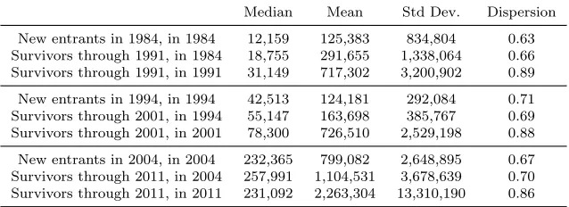
Table 8 reports the median, mean, standard deviation, and quartile coefficient of dispersion
of nine distributions of interest (each of the three cohorts is associated with three distributions)
mentioned in the previous paragraph. The quartile coefficient of dispersion is a robust measure
of dispersion and is defined as (Q3 −Q1)/(Q3 +Q1), where Q1 and Q3 are the first and the
third quartiles of each dataset. Figure 3 presents the kernel density functions of the nine sets of
log-transformed market capitalization, each panel corresponding to one of the three cohorts. Comparing
the solid curves (All, 1984/1994/2004) with the dashed curves (Survivors, 1984/1994/2004), we
find that stocks that survived through the seven-year tracking period tend to have larger market
capitalization going back in the year of issuance. Comparing the dashed curves with the dotted
curves (Survivors, 1991/2001/2011), we observe that the market capitalization distribution moves
to the right and becomes more dispersed as stocks become mature. The increasing dispersion in
market capitalization distribution is also evident according to the last column in Table 8. Note that
the graphs in Figure 3 use the log of size and the actual dispersion in dollar terms is considerably
greater. Therefore we conclude that the effect of aging on market capitalization distribution is
two-fold. The market capitalization on average becomes larger as time passes. However the market
capitalization distribution also becomes significantly more disperse over time as well. Therefore it
is possible for a stock to be both senior in terms of age and small in terms of market capitalization.
3.6. Return Skewness within Age and Size Decile Groups
In this subsection we examine the skewness of the stock return distribution for different age
and size deciles and discuss the implications for our results. Bessembinder (2018) studied the
distributions of monthly buy-and-hold stock returns in different size decile groups. According to his
Table 8: Summary of three market capitalization distributions for three cohorts of stocks. Market capitalization of three cohorts of stocks, namely those entered the CRSP database in 1984, 1994, and 2004, are tracked over a seven-year period after their entrance. Each cohort is associated with three market capitalization distributions of interest. The first one is the distribution among all entrants at the beginning of the tracking period; the second one is the distribution among survivors at the end of the tracking period; the third one is the distribution at the beginning of the tracking period of those stocks that survived until the end of the tracking period. We report the mean, median, standard deviation, and quartile coefficient of dispersion of each distribution for each cohort.
Median Mean Std Dev. Dispersion
New entrants in 1984, in 1984 12,159 125,383 834,804 0.63 Survivors through 1991, in 1984 18,755 291,655 1,338,064 0.66 Survivors through 1991, in 1991 31,149 717,302 3,200,902 0.89
New entrants in 1994, in 1994 42,513 124,181 292,084 0.71 Survivors through 2001, in 1994 55,147 163,698 385,767 0.69 Survivors through 2001, in 2001 78,300 726,510 2,529,198 0.88
New entrants in 2004, in 2004 232,365 799,082 2,648,895 0.67 Survivors through 2011, in 2004 257,991 1,104,531 3,678,639 0.70 Survivors through 2011, in 2011 231,092 2,263,304 13,310,190 0.86
from small to big groups. However themean return in each size group does not show a clear pattern except that the smallest group yields a mean return much higher than any other size group. This
observation implies that the observed “small firm effect" is to a large extent a result of the extreme
positive skewness in the smallest 10% of firms. Another important implication of this finding is that
heterogeneity in the smallest 10% of firms in terms of return is unmatchable by that in any other
size group. Since stock age is a key feature in our study, it is also of interest to explore the pattern
in the within-group skewness when stocks are grouped by age.
The leftmost columns of Table 9 report the mean, median, and skewness of monthly
buy-and-hold stock returns grouped by size and the rightmost columns report the the set of statistics when
the stocks are grouped by size. For each month during the period from January 1977 to December
2016 each available stock is assigned to a size (age) decile group based on its market capitalization
(age since issuance) at the end of the last month. A group number closer to 10 means a more
senior group or a larger-cap group. In this way each stock-month combination is tagged with an
age group number and a size group number. Each decile group contains roughly 10% of the
stock-month observations. Each stock-stock-month observation is associated with a buy-and-hold return20 of
the particular stock over the particular month. The reported statistics are calculated based on all
annualized monthly returns that belong to each decile group. The first four columns in Table 9
report similar information to that reported in Table 3A - Panel A of Bessembinder (2018). The
20
Figure 3: Kernal Density Functions of Log Market Capitalization. Market capitalization of three cohorts of stocks, namely those entered the CRSP database in 1984, 1994, and 2004, are tracked over a seven-year period after their entrance. Each cohort is associated with three market capitalization distributions of interest. The first one is the distribution among all entrants at the beginning of the tracking period; the second one is the distribution among survivors at the end of the tracking period; the third one is the distribution at the beginning of the tracking period of those stocks that survived until the end of the tracking period. Each panel in the figure corresponds to an indicated cohort, and the kernel density functions of the three distributions of log market capitalization are shown.
the data used21.
Despite the difference in source data the pattern in return skewness across different decile groups
shown in Table 9 is similar to that reported in Bessembinder’s study: extremely positive skewness is
observed in the smallest decile group, and there is a decreasing trend in the within-group skewness
as we move from small to big size groups. The last four columns in Table 9 show the return statistics
in different age decile groups. Compared with what we can observe from the within-group mean
returns in different size groups, here we can see a more distinctly increasing trend in the within-group
mean return as we move from young to senior age groups. However it is worth noting that the mean
returns in the youngest and in the second youngest decile groups are reversely ordered compared
with the general trend; this is also true in the comparison between the oldest and second oldest decile
groups. A potential explanation for both observations can be found from the industrial organization
literature. Fichman and Levinthal (1991) explain why firms face an initial “honeymoon" period in
which they are buffered from a sudden exit by their initial stock of resources. Barron et al. (1994)
argue that old firms are prone to suffer from a “liability of obsolescence" and also a “liability of
senescence". This effect will be discussed in more detail in Section 4.
There is a marked difference in the skewness patterns in the size decile and in the age decile. For
the size decile the return skewness decreases as we move in the direction of increasing firm size with
the smallest decile having a skewness of 6.08 and the largest decile having a skewness of just 0.41.
For the age decile the return skewness is remarkably stable with an average value of5.07 across all
age groups.
If we assign stocks to decile groups based on an ideal (hypothetical) factor, then the conditional
return distribution in different groups should be clearly distinct. The overall return distribution is
a mixture of ten distinct conditional distributions. In such a scenario we should expect a monotonic
trend in the within-group mean and reduced (compared with skewness of unconditional return
dis-tribution) within-group skewness. Figure 4 shows a hypothetical unconditional return distribution
and illustrates the effect of grouping according to different factors on the within-group (conditional)
mean and skewness. The effect of grouping according to an ideal factor on within-group mean and
21
Figure 4: All three panels show a same histogram of hypothetical stock returns. We intend to illustrate the effect of factor-based grouping on within-group mean and skewness. In each panel, different bins are colored differently to reflect the level of factor. A darker blue color represents a more favorable factor group in the top panel, a more senior age group in the middle panel, and a bigger size group in the bottom panel.
Density
0.0
0.2
0.4
0.6
0.8
Illustration of an ideal factor
return
Most negative Most positive
Density
0.0
0.2
0.4
0.6
0.8
Illustration of the age factor
return
Youngest Oldest
Density
0.0
0.2
0.4
0.6
0.8
Illustration of the size factor
return
skewness is illustrated in the top panel of Figure 4. Here a darker color stands for a more favorable
factor group. According to Table 9 neither factor appears to be that ideal. For the age factor
monotonicity is roughly observed but the conditional distributions are quite skewed. The middle
panel of Figure 4 illustrates such a possibility. Here a darker color represents a more senior age
group. For the size factor the monotonicity is violated. However most within-group skewness is
reduced compared with skewness of the unconditional distribution of 5.13. This effect is illustrated
in the bottom panel of Figure 4. Our key results depend more on the monotonicity feature and are
[image:29.612.141.471.327.443.2]not affected much by the skewness feature since skewness can be diversified away in portfolios.
Table 9: Statistics of one-month buy-and-hold returns in different size and age decile groups. For each month during the period from January 1977 to December 2016, each available stock is assigned to a size (age) decile group based on its market capitalization (age since issuance) at the end of the last month. A group number closer to 10 means a more senior group or a larger-cap group. Each stock-month observation is associated with a buy-and-hold return of the particular stock over the particular month. The reported statistics are calculated based on all annualized monthly returns that belong to each decile group.
Size Group Mean Median Skew Age Group Mean Median Skew
1 0.2883 0.0000 6.0821 1 0.0988 0.0000 2.8856
2 0.1008 0.0000 3.3851 2 0.0825 0.0000 5.5759
3 0.0981 0.0000 3.1559 3 0.1131 0.0000 5.8414
4 0.1109 0.0000 3.5532 4 0.1543 0.0000 4.4354
5 0.1208 0.0000 2.4979 5 0.1254 0.0000 5.2705
6 0.1259 0.0000 1.8118 6 0.1766 0.0000 5.8495
7 0.1313 0.0593 1.3073 7 0.1589 0.0000 4.2460
8 0.1384 0.0945 1.2735 8 0.1624 0.0027 5.0487
9 0.1344 0.1126 0.7520 9 0.1575 0.0550 4.5711
10 0.1249 0.1173 0.4136 10 0.1400 0.0938 6.9448
4. Understanding Stock Age Effects
Many economic theories tend to treat firm size and firm age as capturing the same fundamental
information. For example Greiner (1989) presents his “stages of growth" model of organizational
change in growing firms, in which size is linearly related to age. Other scholars have nonetheless
made specific predictions about how firm performance changes with age. In this section we review
these theoretical predictions in terms of three categories: selection effects, learning-by-doing effects,
and inertia effects.
It is worth pointing out that the stock age used in our study is calculated based on the date on
which a stock appears in the CRSP database for the first time. The three effects to be reviewed are
from the industrial organization literature and characterize firms’ earning ability in different stages.
capable of explaining the stock age effects we have discovered and therefore briefly discuss them
since they may help explain some of the key findings in this paper.
4.1. Selection Effects
Selection effects arise when selection pressures progressively eliminate the weakest firms, and
result in an increase in the average productivity level of surviving firms, even if the productivity
levels of individual firms do not change with age. This situation corresponds to an influential model
in Industrial Organization in Economics proposed by Jovanovic (1982). According to this model,
firms are born with fixed productivity levels, and learn about their productivity levels as time passes.
In this model, low productivity firms are observed to exit, while high productivity firms remain in
business. As a result the average productivity of the cohort increases with the cohort ages, even
if the productivity levels of individual firms remain constant over time. Therefore selection effects
provide a potential explanation for the age effect uncovered in our study.
4.2. Learning-by-doing Effects
Learning-by-doing effects occur when firms increase their productivity as they learn about more
productive production techniques and incorporate these improvements in their production routines.
(See Ulen and Newman (1998) for a survey of the learning-by-doing concept.) Learning-by-doing
effects can be expected to be particularly relevant for young firms. According to Garnsey (1998):
“New firms are hampered by their need to make search processes a prelude to every new problem
they encounter. As learning occurs benefits can be obtained from the introduction of a repertoire of
problem-solving procedures ... eliminating open search from the problem-solving response greatly
reduces the labor and time required to address recurrent problems."
Furthermore older firms may benefit from their greater business experience, established contacts
with customers, and easier access to resources. For example, Sørensen and Stuart (2000) point out
that entrepreneurs often lack detailed information about their jobs, firms and even the environments
until they are active in the market. After a firm’s creation, an intense learning process starts
and contributes to the firm’s growth and survival in the long-term. Also Chang et al. (2002)
provide evidence on the existence of microeconomic “learning-by-doing" effects with positive effects
on the aggregate output. The learning-by-doing effects may provide an explanation to the positive