http://www.scirp.org/journal/tel ISSN Online: 2162-2086
ISSN Print: 2162-2078
DOI: 10.4236/tel.2017.76125 Oct. 30, 2017 1834 Theoretical Economics Letters
Influence of Oil Price Volatility of Developed
Countries on Emerging Countries Stock Market
Returns by Using Threshold Based Approach
Kirti Arekar, Rinku Jain
K.J. Somaiya Institute of Management Studies & Research, Mumbai, India
Abstract
This study reveals the nonlinear relationship between oil price volatility of the developed countries and emerging stock market returns. We analyzed the ef-fects of oil price volatility of the developed markets i.e. India, United States and United Kingdom on the emerging stock market returns. We used VAR, Granger Causality, impulse responses and logistic transition based autore-gressive model (LSTR) in two groups. In group one, we considered US oil price volatility with six emerging countries and regions stock market returns
i.e. France, Spain, Malaysia, Japan, Singapore and Taiwan. In group two, we considered oil price with respect to India with the same six emerging coun-tries stock market returns. The data covers the daily closing prices for seven years from 2011 to 2017 for emerging countries and for oil prices the data we use West Texas Intermediate (WTI) spot price of crude oil for US and India. This study helps the investors to understand the impact of oil prices of US and Indian market with respect to emerging markets and whether to identify the dependency of emerging stock markets returns on the oil prices of US and In-dia. All the analysis was performed by using R and EVIEWS software.
Keywords
Logistic Transition Based Autoregressive Model (LSTR), Non-Linear, Vector Decomposition Method, Emerging Markets
1. Introduction
Oil price volatility dynamics have significant economic impact in emerging stock market returns. Jones and Kaul [1] study the impact of oil prices on stock mar-ket returns using vector autoregressive approach (VAR). The oil prices have an How to cite this paper: Arekar, K. and
Jain, R. (2017) Influence of Oil Price Vola-tility of Developed Countries on Emerging Countries Stock Market Returns by Using Threshold Based Approach. Theoretical Economics Letters, 7, 1834-1847.
https://doi.org/10.4236/tel.2017.76125
Received: September 29, 2017 Accepted: October 27, 2017 Published: October 30, 2017
Copyright © 2017 by authors and Scientific Research Publishing Inc. This work is licensed under the Creative Commons Attribution International License (CC BY 4.0).
http://creativecommons.org/licenses/by/4.0/
DOI: 10.4236/tel.2017.76125 1835 Theoretical Economics Letters impact of real economy activity include both supply and demand channels and it also affects the consumption and investment. Consumption is affected by the disposable income. As the oil price increases consumers spending power de-creases and therefore it will affect the investment decisions. In this study, we analyzed the effects of oil price volatility of US and India on the different emerging stock market returns. We employed VAR, Granger Causality, impulse responses and logistic transition based autoregressive model (LSTR).
Sadorsky [2] and Papapetrou [3] found negative relationship between US and Greece stock market returns with oil prices shocks. O’Neil et al. [4] found that rise in oil prices will lead to reduce stock market prices for US, UK and France. Park and Ratti [5] considered 12 European oil importing countries. Masih et al. [6] studies the volatility impact of oil price on stock market return in Korea and the results estimated that there are the strong effects of oil price volatility on real stock market returns. Creti et al [7] identified the relationship between 25 com-modities including crude oil and stocks. Choi and Hammoudeh [8] investigated the relationship between commodity price and S & P 500 index which shows the increasing correlation between all the commodities. Bwo Nung Huang [9] ap-plied the multivariate threshold model to investigate the impact of oil price change and its volatility on economic activity. He explained that the change in oil price are the better estimators of the explain macro-economic variables then the volatility of the oil price.
Huson Joher [10] considered the existence of a no linear relationship between oil price volatility and equity market uncertainty. He concludes that some sec-tors are responding quickly to volatility. John Elder et al. [11] studied the effects of oil price uncertainty in Canada and their study exposes that ambiguity about oil prices incline to emphasize the negative reaction of output to positive oil shocks. Evangelia (2009) considered the connection between oil prices and eco-nomic movement in Greece during the period 1982 to 2008. Her research finds that there is a negative correlation between oil prices and economic activity during periods of rapid oil price changes and high oil price change volatility.
Guo and Kliesen [12] investigates that daily crude oil price has a negative ef-fect on future GDP growth and other methods of the US macro economy. Zhang [13] developed nonlinear relationship between oil price shock and economic growth in Japan. Lardic and Mignon [14] studied the nonlinear term relation-ship between US and Europe economy. Our study provided the new under-standing that how the oil price of US and Indian responds the stock market re-turns of emerging countries. We had used threshold autoregressive approach which is expected to add a new paradigm in the oil prices and stock market vola-tility relationship literature.
DOI: 10.4236/tel.2017.76125 1836 Theoretical Economics Letters
2. Empirical Models
Logistic transition based auto regressive model (LSTR) defined by Teravirta and Anderson [15] and Teravirta [16] estimates at which transition take place from one regimes (lower level effect of oil price volatility on India and Us market) to another( higher level effect on stock market volatility of emerging market dy-namics). In this study, in group one two dynamics regimes are used first is the oil price volatility of the US market and the other stock market index and term spread is considered. The mathematical model for group 1 is as follows:
(
)
10 1 1 1 20 2 2 2
1 1
; ,
p p
t jt j t t jt j t t t t
j j
f TS f TS h f c
η θ
θ
−λ
ς
θ
θ
−λ
ς
γ
ε
= =
= + + + + + + + +
∑
∑
(1)where, ηt is the rolling standard deviation over 12 months for respective
emerging countries stock market index and ft is the transition variables i.e. oil
price return volatility for US market. In emerging market stock index for each country has two regimes with respect to oil price uncertainty namely high and low volatility regimes where h f
(
t; ,γ c)
is the transition function bounded by the value 0 and 1. C is considered as the threshold parameter; γ represent the speed and smoothness of the transition. The control variable term is introduced to understand the effect of external factors on the emerging stock market index.In group two, two dynamics regimes are used first is the oil price volatility of the Indian market and the other stock market index and term spread is consi-dered. The mathematical model for group 1 is as follows:
(
)
10 1 1 1 20 2 2 2
1 1
; ,
p p
t jt j t t jt j t t t t
j j
f TS f TS h f c
µ θ
θ
−λ
ς
θ
θ
−λ
ς
γ
ε
= =
= + + + + + + + +
∑
∑
(2)where, µt is the rolling standard deviation over 25 days for respective emerging
countries stock market index and ft is the transition variables i.e. oil price
re-turn volatility for Indian market. In emerging market stock index for each coun-try has two regimes with respect to oil price uncertainty namely high and low volatility regimes where h f
(
t; ,γ c)
is the transition function bounded by the value 0 and 1. C is considered as the threshold parameter; γ represent the speed and smoothness of the transition. The control variable term is introduced to understand the effect of external factors on the emerging stock market index.Two specific forms of the transition function h f
(
t; ,γ c)
are used for both the groups (see Teravirta and Anderson, 1992 and Terasvitra, 1994):LTST 1
(
)
(
(
(
)
)
)
11 t; , 1 exp t ; 0
h f γ c = + −γ f −c − γ >
LTST 2
(
)
(
(
(
)
2)
)
2 t; , 1 exp t ; 0
h f
γ
c = + −γ
f −cγ
>To test linearity against LSTR, Langrange multiplier (LM) to test the hypothe-sis of no-nonlinear relationship as given by Terasvitra (1994). λ1 and λ2 will
dis-DOI: 10.4236/tel.2017.76125 1837 Theoretical Economics Letters turbances on the system of variables. An impulse response is used to identify the shock to the i-th variable not only directly affects the i-th variable but is also transferred to all of the other endogenous variables through the dynamic (lag) structure of the VAR.
Methodology
The empirical analysis in this paper is based on daily stock market returns for six emerging countries and oil price volatility for US and Indian market. The data considered from the period April, 2011 to Ferburary 2017 with 1457 daily ob-servation for each emerging countries and regions stock market index i.e.
France, Spain, Malaysia, Japan, Singapore and Taiwan. Data for stock market index of respectively emerging countries are obtained from Bloomberg and to measure oil price volatility we used West Texas Intermediate (WTI) spot price of crude oil. All the analysis is carried out by using R and EVIEWS software.
3. Findings
3.1. Volatility Fluctuation
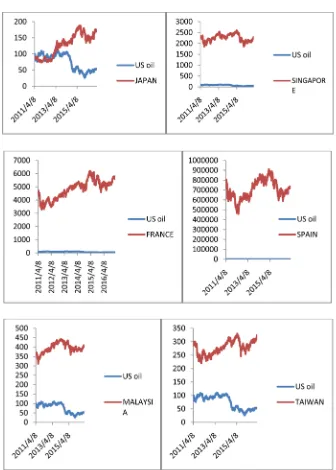
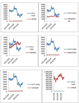
From Figure 1, it is observed that for the emerging countries i.e. France, Singa-pore and Spain have high volatility as compared with other emerging countries. And, for the Japan there is lower level of volatility. Overall, stock market index for all emerging countries seems to be consistently higher than the US oil price because the returns of all the emerging market countries are higher than the US oil prices. And. From Figure 2, we identified that for the emerging countries and regions i.e. Japan, Taiwan and Malaysia have higher volatility as compared with other countries. The France and Singapore has a lower level of volatility with respect to oil prices of India. And overall, stock market stock market index for all emerging countries seems to be consistently higher than oil prices volatility of India expect Spain. This relationship helps us to understand the volatility pattern between US and India oil prices with emerging countries stock index.
3.2. Vector Auto Regressive Analysis
VAR analysis is divided into three parts i.e. Granger Causality and Vector De-composition method. To understand the causal relation between the stock mar-ket returns of emerging marmar-ket and oil price volatility of oil prices of US and In-dia we use granger Casualty test.
The results from granger causality test from VAR model is reported in Table 1 and Table 2. Table 1 will represent the causal effect between oil price volatility of US and stock market index of emerging countries. Null hypothesis of no cau-sality got rejected for the countries and regions Taiwan, Malaysia and Japan and for the remaining three countries null hypothesis of no causality do not rejected. So, oil price volatility of US market has Granger cause with the stock market in-dex of emerging countries and regions like Taiwan, Malaysia and Japan.
DOI: 10.4236/tel.2017.76125 1838 Theoretical Economics Letters
Figure 1. Volatility pattern between US oil price and Emerging countries and regions stock Index.
Table 1. The effect between oil price volatility of US and stock market index of emerging countries and regions.
Emerging Countries and regions Stock Market Test Value p-Value
France 0.124 0.321
Spain 0.254 0.789
Singapore 0.005 0.567
Taiwan 3.231 0.002
Malaysia 5.654 0.000
[image:5.595.201.540.604.731.2]DOI: 10.4236/tel.2017.76125 1839 Theoretical Economics Letters
Figure 2. Volatility pattern between India oil price and emerging countries and regions stock Index.
Table 2. Represent the causal effect between oil price volatility of India and stock market.
Emerging Countries and regions Stock Market Test Value p-Value
France 9.82 0.0073
Spain 7.52 0.0232
Singapore 0.425 0.8083
Taiwan 0.183 0.9128
Malaysia 2.56 0.2793
Japan 0.232 0.8903
[image:6.595.208.539.559.679.2]DOI: 10.4236/tel.2017.76125 1840 Theoretical Economics Letters null hypothesis of no causality do not rejected. So, oil price volatility of Indian market has Granger cause with the stock market index of emerging countries like France, and Spain.
3.3. Impulse Response
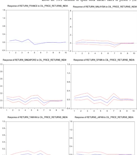
A shock to the i-th variable not only directly affects the i-th variable but is also transmitted to all of the other endogenous variables through the dynamic (lag) structure of the VAR. An impulse response function traces the effect of a one- time shock to one of the innovations on current and future values of the endo-genous variables. The impulse response for US oil prices and oil prices of India with respect to all other emerging countries stock index are shown in Figure 3 and Figure 4.
Figure 3 and Figure 4 show the impulse response function curves of real stock returns of emerging from a one standard deviation shock of the Indian oil price volatility and stock returns of emerging countries. Mostly an impulse re-sponse function dashes the effect of a one-time shock to one of the innovations on current and future values of the endogenous variables.
In Figure 3, a one standard deviation shock to Indian oil price volatility causes significant positive response for 4 days periods in France and Spain, 5 days periods in Malaysia and 3 days periods in Singapore stock index volatility. Whereas Japan stock index volatility displays an extended negative response lastly beyond 5 days resulting the Indian oil price volatility shock. If there is one standard deviation positive change in Indian oil price, Taiwan stock return volatility will response negatively increase till two days period and after five days period, it shows positive response. One unit increase in oil price volatility, will increase the Japan index re-turn by 6% in days 1 period, and Taiwan index rere-turn by 3% in days 3 period.
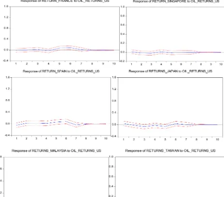
In Figure 4, a one standard deviation shock to US oil price volatility causes significant positive response for 4 to 8 days periods in France, 2 to 7 days period in Spain, 1 to 7 days period in Malaysia stock index volatility. Whereas Japan stock index volatility displays an extended negative response for 1 to 7 days pe-riods. One unit increase in US oil price volatility causes negative response in 2 to 4 days period and 5 to 6 days period in Taiwan stock index volatility. Singapore stock index market will not show any response due to one unit shock in US oil price volatility. One unit increase in US oil price volatility, will increase the France index return by 9% and Spain index return by 3% in days 6 period.
3.4. Vector Decomposition
Variance decomposition separates the variation in oil prices of US and India with respect to the stock market index for six emerging countries into the component shocks to the VAR. Thus, the variance decomposition provides information about the relative importance of each random innovation in affecting the variables in the VAR. Table 3 and Table 4 represent the variance decomposition of oil prices of US and India in the model with stock market index of six emerging countries.
DOI: 10.4236/tel.2017.76125 1841 Theoretical Economics Letters France stock market index in period 3(i.e. short run shocks) but it will increased for period 12 (in long run shock) i.e. 0.79% variation. US oil price volatility shows the 3.8% variation in Spain stock market index in period 3 (i.e.
DOI: 10.4236/tel.2017.76125 1842 Theoretical Economics Letters
[image:9.595.57.540.597.728.2]Figure 4. Impulse response function curves of real stock returns of emerging from a one standard deviation shock of the Indian oil price volatility and stock returns of emerging countries and regions.
Table 3. Variance decomposition of US oil price with other emerging countries and regions.
Period Variance decomposition of US oil prices due to shocks
US Oil France Spain Malaysia Singapore Taiwan Japan
3 99.023(0.6123) *** (0.0911) 0.0068 (0.1612) 0.038 (0.242) 0.086 (0.262) 0.1615 (0.315) 0.350 (0.412) 0.333
6 99.008(0.6321) *** (0.0910) 0.0076 (0.175) 0.045 (0.243) 0.087 (0.2622) 0.1616 (0.316) 0.350 (0.418) 0.345
9 99.001(0.623) *** (0.0910) 0.0076 (0.173) 0.045 (0.244) 0.0876 (0.2623) 0.1616 (0.316) 0.350 (0.173) 0.345
DOI: 10.4236/tel.2017.76125 1843 Theoretical Economics Letters
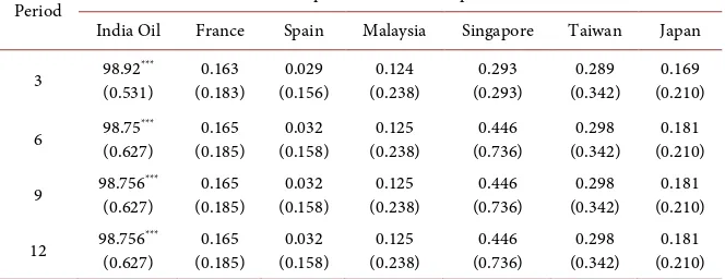
Table 4. Variance decomposition of India oil price with other emerging countries and re-gions.
Period Variance decomposition of India oil prices due to shocks
India Oil France Spain Malaysia Singapore Taiwan Japan
3 98.92(0.531) *** (0.183) 0.163 (0.156) 0.029 (0.238) 0.124 (0.293) 0.293 (0.342) 0.289 (0.210) 0.169
6 98.75(0.627) *** (0.185) 0.165 (0.158) 0.032 (0.238) 0.125 (0.736) 0.446 (0.342) 0.298 (0.210) 0.181
9 98.756(0.627) *** (0.185) 0.165 (0.158) 0.032 (0.238) 0.125 (0.736) 0.446 (0.342) 0.298 (0.210) 0.181
12 98.756(0.627) *** (0.185) 0.165 (0.158) 0.032 (0.238) 0.125 (0.736) 0.446 (0.342) 0.298 (0.210) 0.181
short run shocks) but it will increased for period 12 (in long run shock) i.e. 4.6% variation. US oil price volatility shows the 8.6% variation in Malaysia stock market index in period 3 (i.e. short run shocks) but it will increased for period 12 (in long run shock) i.e. 8.7% variation. US oil price volatility shows the 16.15% variation in Singapore stock market index in period 3 (i.e. short run shocks) but it will increased for period 12 (in long run shock) i.e. 17.5% varia-tion. US oil price volatility shows the 35.0% variation in Taiwan stock market index in period 3 (i.e. short run shocks) but it will increased for period 12 (in long run shock) i.e. 35.2% variation. US oil price volatility shows the 33.3% variation in Japan stock market index in period 3 (i.e. short run shocks) but it will increased for period 12 (in long run shock) i.e. 35.6% variation. US oil prices also shows the significant variation in the stock market index of all emerging countries in both short and long run shocks. It is also observed that maximum variation occurs in Japan stock market index due to the variation in the US oil prices and minimum variation occurs in France stock market in short and long run periods.
From the above table it is clear, INDIA oil price volatility shows the 16.3% variation in France stock market index in period 3(i.e. short run shocks) but it will increased for period 12 (in long run shock) i.e. 16.5% variation. INDIA oil price volatility shows the 2.9% variation in Spain stock market index in period 3 (i.e. short run shocks) but it will increased for period 12 (in long run shock) i.e.
DOI: 10.4236/tel.2017.76125 1844 Theoretical Economics Letters emerging countries in both short and long run shocks. It is also observed that maximum variation occurs in Singapore stock market index due to the variation in the India oil prices and minimum variation occurs in Spain stock market in short and long run periods.
4. LSTR Model
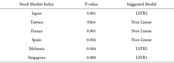
The LSTR model gives the linearly test based on Terasvirta and Andeson, 1992 and Terasvitra, 1994 for emerging stock market index with respect to US and Indian oil price volatility. From Table 5, it is observed that for Singapore, Japan and Taiwan stock market index null hypothesis of no lineratity is rejected with respect to US oil price volatility. For Japan and Taiwan we used LSTR 2 model and for Singapore we used LSTR1. From Table 6, it is observed that for Singa-pore, Japan and Malaysia stock market index null hypothesis of no lineratity is rejected with respect to Indian oil price volatility. For Japna and Malaysia we used LSTR 2 model and for Singapore we used LSTR1.
LSTR Model Estimates
The LSTR estimates wer reported in Table 7 and Table 8, for US and India Oil price Voalatility. A a first step, we test linear and non-liner parts (λ1 and λ2),
[image:11.595.207.540.449.568.2]which determined the relationship between US oil price volatility and emerging stock market index. In non-liner regime the Singapore stock market index is significantly positive so we can say that Singapore stock market index tends to increase, with an increase in US oil return volatility and it is also stastically sig-
Table 5. Linearity Test against LSTR Model (US oil price Volatility).
Stock Market Index P-value Suggested Model
Japan 0.001 LSTR2
Taiwan 0.003 LSTR2
France 0.084 Non Linear
Spain 0.756 Non Linear
Malaysia 0.522 Non Linear
Singapore 0.000 LSTR1
Table 6. Linearity Test against LSTR Model (Indian oil price Volatility).
Stock Market Index P-value Suggested Model
Japan 0.001 LSTR2
Taiwan 0564 Non Linear
France 0.891 Non Linear
Spain 0.056 Non Linear
Malaysia 0.004 LSTR2
[image:11.595.208.538.600.721.2]DOI: 10.4236/tel.2017.76125 1845 Theoretical Economics Letters
Table 7. LSTR Estimates using US oil Price Volatality.
Stock
Index MODEL LSTR λ1 TS λ2 TS C1 C2 γ
Japan 2 (−0.71) 0.007 (−0.15) −0.016 (−0.38) 0.451 (0.000)0.187 *** (−0.90) 12.05 (0.00)16.38 *** (0.911) 8.75
Taiwan 2 (0.001)0.032 *** (0.000)−0.021 *** (−0.75) −0.033 (−0.77) 0.346 (0.000)15.25 *** (0.00)17.35 *** (0.049) 1.42
Singapore 1 (0.000)−0.561 *** (0.000)0.120 *** (0.000)0.496 *** (0.000)−0.139 *** (0.000)9.17 *** (0.07)46.01 *
Note: The table follows the following LSTR model
( )
10 1 1 1 20 2 2 2
1 1
; ,
p p
t j t j t t j t j t t t t
j j
f TS f TS h f c
η θ θ − λ ς θ θ − λ ς γ ε
= =
= + + + + + + + +
∑
∑
. ***, **,* denotesstatis-taclly significant at 1%, 5% and 10% level respectively.
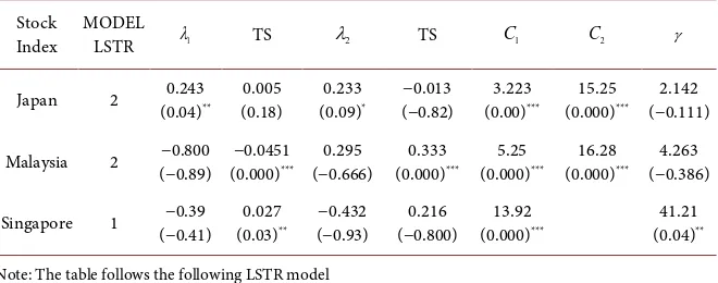
Table 8. LSTR Estimates using Indian oil Price Volatality.
Stock
Index MODEL LSTR λ1 TS λ2 TS C1 C2 γ
Japan 2 (0.04)0.243 ** (0.18) 0.005 (0.09)0.233 * (−0.82) −0.013 (0.00)3.223 *** (0.000)15.25 *** (−0.111) 2.142
Malaysia 2 (−0.89) −0.800 (0.000)−0.0451 *** (−0.666) 0.295 (0.000)0.333 *** (0.000)5.25 *** (0.000)16.28 *** (−0.386) 4.263
Singapore 1 (−0.41) −0.39 (0.03)0.027 ** (−0.93) −0.432 (−0.800) 0.216 (0.000)13.92 *** (0.04)41.21 **
Note: The table follows the following LSTR model
( )
10 1 1 1 20 2 2 2
1 1
; ,
p p
t j t j t t j t j t t t t
j j
f TS f TS h f c
µ θ θ − λ ς θ θ − λ ς γ ε
= =
= + + + + + + + +
∑
∑
. ***, **, * denotesstatis-taclly significant at 1%, 5% and 10% level respectively.
nificant. In a linear regime, Taiwan and Singapore shows the negative relation-ship and statistically significant.
Thirdly, it is clearly observed that Singapore retain LSTR1 form, the stock market volatility of Singapore is significantly affected if the oil price of US in-credsed at ceratain threshold level. However, Japan and Taiwan return LSTR 2. Japan and Taiwan stock market returns are highly sensitive when oil return vo-latility falls under the lower and upper levels of the threshold estimates. Forth, the value of stock parameter γ, for Singapore stock market index is higher i.e.
46.01. Taiwan and Japan stock market index exhibits smoother transition with the γ value 8.75 and 1.42.
In non-liner regime, the Japan stock market index is significantly positive so we can say that Japan stock market index tends to increase, with an increase in Indian oil return volatility and it is also stastically significant. In a linear regime, Malaysia and Singapore shows the negative relationship and statistically signifi-cant.
[image:12.595.209.539.292.422.2]in-DOI: 10.4236/tel.2017.76125 1846 Theoretical Economics Letters credsed at certain threshold level. However, Japan and Malaysia return LSTR 2. Japan and Malaysia stock market returns are highly sensitive when oil return volatility falls under the lower and upper levels of the threshold estimates. Forth, the value of stock parameter γ, for Singapore stock market index is higher i.e.
41.21. Malaysia and Japan stock market index exhibits smoother transition with the γ value 4.623 and 2.142.
5. Conclusion
The findings of this study are significantly useful for the investors. For the emerging countries and regions France, Singapore and Spain show the high vo-latility with respect to US oil prices whereas for India Japan, Malaysia and Tai-wan show the higher volatility. The findings are helpful for making an invest-ment globally and to understand the investinvest-ment pattern of all selected emerging stock market index. By using volatility threshold, investors formulate the short and long term investment plans. Oil price volatility of US market has Granger cause with the stock market index of emerging countries and regions like Tai-wan, Malaysia and Japan and oil price volatility of Indian market has Granger cause with the stock market index of emerging countries like France, and Spain. There are total 23 emerging countries were dealing in the stock market, but in our study, we included only six emerging countries stock index, so this study cannot claim a global representation. Further, studies are suggested to include more emerging stock markets to gain more global market relationship with oil prices volatility.
6. Limitations
There are total 23 emerging countries which deal in the stock market. The major limitations of the study is that we included only six emerging countries but there is the further scope to considered remaining 17 emerging countries. We had also not taken into consideration oil exporting countries. Further, there is the scope to use different financial models i.e. GARCH, T GARCH and E GARCH etc to test the linearly of the stock returns.
References
[1] Jones, C. and Kaul, G. (1996) Oil and the Stock Markets. Journal of Finance, 11, 463-491. https://doi.org/10.1111/j.1540-6261.1996.tb02691.x
[2] Sadorsky, P. (1999) Oil Price Shocks and Stock Market Activity. Energy Economics, 21, 449-469. https://doi.org/10.1016/S0140-9883(99)00020-1
[3] Papapetrou, E. (2001) Oil Price Shocks, Stock Market, Economic Activity and Em-ployment in Greece. Energy Economics, 23, 511-532.
https://doi.org/10.1016/S0140-9883(01)00078-0
[4] O'Neil, T.J., Penn, J. and Terrell, R.D. (2008) The Role of Higher Oil Prices: A Case of major Developed Countries. Research in Finance, 24, 287-299.
https://doi.org/10.1016/S0196-3821(07)00211-0
DOI: 10.4236/tel.2017.76125 1847 Theoretical Economics Letters
13 European Countries. Energy Economics, 30, 2587-2608.
https://doi.org/10.1016/j.eneco.2008.04.003
[6] Masih, R., Peter, S. and Mello, L.D. (2011) Oil Price Volatility and Stock Price Fluc-tuation in an Emerging Market: Evidence from South Korea. Energy Economics, 33, 975-986. https://doi.org/10.1016/j.eneco.2011.03.015
[7] Creti, A., Joets, M. and Mignon, V. (2013) On the Links between Stock and Com-modity Markets’ Volatility. Energy Economics, 37, 16-28.
https://doi.org/10.1016/j.eneco.2013.01.005
[8] Choi, K. and Hammoudeh, S. (2010) Volatility Behavior of Oil, Industrial Com-modity and Stock Markets in a Regime-Switching Environment. Energy Policy, 38, 4388-4399. https://doi.org/10.1016/j.enpol.2010.03.067
[9] Huang, B.-N., Hwang, M.J. and Peng, H.-P. (2005) The Asymmetry of the Impact of Oil Price Shocks on Economic Activities: An Application of the Multivariate Thre-shold Model. Energy Economics, 27, 455-476.
[10] Ali Ahmed, H.J. (2017) Oil Price Volatility and Sectoral Returns Uncertainty: Evi-dence from a Threshold Based Approach for the Australian Equity Market. Journal of Developing Areas, 51, 329-342.https://doi.org/10.1353/jda.2017.0018
[11] Elder, J. and Serletis, A. (2009) Oil Price Uncertainty in Canada. Energy Economics, 31, 852-856.
[12] Guo, H. and. Kliesen, K. (2005) Oil Price Volatility and U.S. Macroeconomic Activ-ity. Federal Reserve Bank of St. Luis, Review 87, No. 6, 669-683.
[13] Zhang, D. (2008) Oil Shock and Economic Growth in Japan: A Nonlinear Ap-proach. Energy Economics, 30, 2374-2390.
[14] Lardic, S. and Mignon, V. (2006) The Impact of Oil Prices on GDP in European Countries: An Empirical Investigation Based on Asymmetric Cointegration. Energy Policy, 30, 3910-3915.
[15] Teräsvirta, T. and Anderson, H.M. (1992) Characterizing Nonlinearities in Business Cycles Using Smooth Transition Autoregressive Models. Journal of Applied Eco-nometrics, 7, 119-136.https://doi.org/10.1002/jae.3950070509