http://www.scirp.org/journal/am ISSN Online: 2152-7393
ISSN Print: 2152-7385
DOI: 10.4236/am.2017.810110 Oct. 31, 2017 1515 Applied Mathematics
The Water Problem and Its Solution in Gansu,
China
Yuke Li
1, Luyi Wang
2, Hai Cheng
31School of International Studies, University of International Business and Economics, Beijing, China 2School of Banking and Finance, University of International Business and Economics, Beijing, China
3School of Information Technology and Management, University of International Business and Economics, Beijing, China
Abstract
Based on such severe situation, we need to work out a way that enables us to analyze the current and future ability of a region to provide clean water to meet the needs of its population, and to develop a reasonable strategy to op-timize the utilization of water resources in this area. This paper has worked out a resolution model and input the data of China, the United States, Russia, Laos and Afghanistan to do national testing. Then, we use the policy from “diaper incident” to do policy testing. The calculation results of the model are in conformity with the reality. Therefore, the model is effective. At last this model is used to resolve Gansu’s water problem and provide effective advices for the local government.
Keywords
Water Scarcity, Water Supply Effect, China Resources Problems
1. Introduction
According to the UN water scarcity map, we find that the northern China is suf-fering from serious water scarcity. Some of the northern provinces in China even have achieved the degree of over-exploited, and Gansu province is included in these provinces. After conducting further investigation, we find that in Gansu province for many years, the average annual production capacity of surface wa-ter is 28.2 billion cubic mewa-ters, which accounts for 1% of the total surface wawa-ter in China and ranks 29th out of 32 provinces (municipalities/ autonomous re-gions). The amount of water per acre reaches 378 cubic meters, which is about only a quarter of the national average and thus belongs to the serious water shortage areas. The per capita water capacity in Gansu is 1077 cubic meters,
How to cite this paper: Li, Y.K., Wang, L.Y. and Cheng, H. (2017) The Water Problem and Its Solution in Gansu, China. Applied Mathematics, 8, 1515-1528.
https://doi.org/10.4236/am.2017.810110
Received: September 11, 2017 Accepted: October 28, 2017 Published: October 31, 2017
Copyright © 2017 by authors and Scientific Research Publishing Inc. This work is licensed under the Creative Commons Attribution International License (CC BY 4.0).
http://creativecommons.org/licenses/by/4.0/
DOI: 10.4236/am.2017.810110 1516 Applied Mathematics which is about one third of the national average, one-eighth of the world’s aver-age and has been close to the international severe water shortaver-age limits.
Therefore, we take Gansu province as a region where water is either heavily or moderately overloaded, which meet the requirements in task 2. We hope to find a way for Gansu province to alleviate water scarcity through this analysis.
2. Model Design
2.1. Model Building
2.1.1. A Brief Introduction of the Model
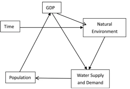
Since a detailed introduction has been stated in “2.1 Outline of the Solution”, thus we only make a simple explanation here as Figure 1.
As shown above, it is a dynamic model of water supply and demand, popula-tion, natural environment, GDP and time. Water supply and demand will have impact on population, and population will change the GDP and GDP per capita. GDP will directly influence the water supply and demand or indirectly influence the water supply and demand by changing the environment. Meanwhile, time is also able to influence the environment and thus change the water supply and demand.
2.1.2. The Operation Mechanism of the Model a) Water Supply and Demand Model:
Water supply (sk) is influenced by natural factors (a_wk) and social facors (ik).
0 1 _ 2
k k k k
s =a + ×a a w + × +a i u
(1)
1) Available water quantity model in the nature:
[image:2.595.250.504.533.707.2]In the nature, available water quantity (a_w) is equal to the total water re-sources (z_w) minus the discharge [1]. In the formula, a0, a1 and a2 are parame-ters that could be determined by the variance between supply (sk) and natural factors (a_wk) and social facors (ik), which is mainly indicated by the investment of water infrastructure, and u_k represents the residual error of the regression model. The model is:
DOI: 10.4236/am.2017.810110 1517 Applied Mathematics
_ _ 10 discharge
a w=z w− × (2)
Since the wastewater is discharged into the nature, it must produce pollution to other water resources. Here we assume that the polluted water is ten times of the sewage discharge.
2) Total water resource model in the nature:
Total water resource (z_wk) in one region is in relation with the local precipi-tation, geology, topography and ecological environment. We assume that the in-fluence of geology and topography to the total water resource is constant. The ability of a region to reserve water is mainly illustrated by forest coverage [2]. And the model is:
0 1 2
_ k precipitationk forest_areak k
z w =b + ×b + ×b +u
(3)
3) Precipitation model:
The atmospheric precipitation water can be calculated by surface vapor pres-sure. With recipitation model, we use surface temperature (T, unit: K) to calcu-late surface saturated vapor pressure (Ew, unit: hPa).
10 10
8.2969 1
4 273 16
273 16 4 76955 1 3
27316
log 10 79574 1 5 02800 log
27316
1 50475 10 1 10
0 42873 10 10 1 0 78614
T T T Ew T − × − − × − = × − − × + × × − + × × − + . . . - . . . . . . . (4)
Then, we use the surface saturated vapor pressure and relative humidity (U, unit: %) to calculate surface vapor pressure.
e=Ew U× (5)
rpressure
U = Ew
(6)
The “rpressure” in the previous formula is the actual vapor pressure, so
rpressure
e=
(7)
Because,
(
)
rpressure=1.25a 1+t 273.15 (8)
“a” is absolute humidity in the previous formula. If a is constant and equals 10 (g/m3), then the precipitation is only related to the temperature. The model is:
2
0 1 2
precipitationk =c + ×c rpressurek+ ×c rpressurek+uk (9)
4) Temperature model:
With greenhouse effect, the temperature tk has the tendency of rising (n represents the year). It is because the growing influence of temperature to the precipitation [3], we build the temperature model:
2 3
0 1 2 3
k k
t =d + × +d n d ×n +d ×n +u (10)
5) Forest area model:
DOI: 10.4236/am.2017.810110 1518 Applied Mathematics influences the local total natural water resources. After consulting materials, the forest area has a strong relation with GDP per capita (gdpk) [4]. We build the forest area model:
2 3
0 1 2 3
forest_areak =e + ×e rgdpk+ ×e rgdpk + ×e rgdpk+uk (11)
6) Investment in water infrastructure model:
Water infrastructure determines whether people can get more water to meet their needs. As is indicated in research, GDP per capita has dramatic impact on the investment in water infrastructure [5]. Imitating the lag variable models, we build this model to illustrate changes of investment in water infrastructure:
0 1
k k k
i = f + ×f rgdp +u
(12)
7) Waste water discharge model:
The amount of waste water discharge
(
rdischargek)
has great influence on the amount of polluted water, which also changes the available water quantity. Referring to EKC research documents, we build this wastewater discharge model based on EKC relationship theory.2 3
0 1 2 3
rdischargek =g + ×g rgdpk+g ×rgdpk +g ×rgdpk+uk (13)
8) Total waste water discharge model:
discharge= ×p rdischarge (14)
b) Water demand model:
Water demand (dk) is not only in relation with population, but also with eco-nomic development. We find the relation between water demand and GDP per capita in research documents, and build this model [6]:
2
0 1 2
k k k k
d = j + ×j rgdp + ×j rgdp +u (15)
c) GDP variation model:
After consulting related documents, we find the close relation between GDP and population (pk). So we build the GDP variation model:
0 1
k k k
gdp =m +m ×p +u (16)
d) Population model:
Because water is significant to human surviving, whether the water supply can meet the needs of water demand has considerable impact on the amount of pop-ulation (pk) [7]. Thus, we build this model:
0 1
k k k
r =z + ×z sd +u (17)
(
)
1 1
k k k
p =p− +r (18)
e) Finally, we use S/D to suggest the ability of a region to provide clean water to meet the needs of its population.
2.2. Model Testing
Application AnalysisDOI: 10.4236/am.2017.810110 1519 Applied Mathematics is accurate and efficient. We get the data of Shandong province from 2005 to 2014 in China’s National Bureau of Statistics, and input these data into the mod-el to conduct the test.
a) Water supply model:
0 1 _ 2
k k k k
s =a + ×a a w + × +a i u (1)
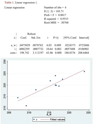
The result of regression analysis is Table 1.
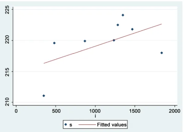
The relationship between sk and a_w is shown in Chart 1. The relationship between sk and I is shown in Chart 2.
As Chart 1 and Chart 2 show, R-squared = 0.9515, which indicates this model explains the changes of s well. Since test value of P by F is close to 0, the model is statistically significant in general, and is moderate fine. Since the estimated value of coefficient of a_w is greater than coefficient of I, it suggests that water supply is more sensitive to the changes of a_w.
198.742 0.0475029 _ 0.0082295
k k k
[image:5.595.223.526.305.705.2]s = + ×a w + ×i (19)
Table 1. Linear regression 1.
DOI: 10.4236/am.2017.810110 1520 Applied Mathematics
[image:6.595.225.525.69.283.2]Chart 2. Available water quantity model (social investment).
Table 2. Linear regression 2.
The coefficient of a_w and I are both positive number, so s is in positive cor-relation with a_w and i.
1) Available water quantity model in the nature:
_ _ 10 discharge
a w=z w− × (2)
2) Total water resource model in the nature:
0 1 2
_ k precipitationk forest_areak k
z w =b + ×b + ×b +u
(3)
The result of regression analysis is Table 2.
The relationship between z_w and precipitation is shown in Chart 3. The re-lationship between z_w and forest_area is shown in Chart 4.
DOI: 10.4236/am.2017.810110 1521 Applied Mathematics
Chart 3. Precipitation and natural water supply.
Chart 4. Forest area and natural water supply.
cipitation. Therefore, the model is:
_ k 149.5273 0.5825711 precipitationk 0.1818078 forest_areak
z w = − + × + × (20)
The coefficient of forest_area and precipitation are both positive number, so
z_w is in positive correlation with precipitation and forest_area. 3) Precipitation model:
2
0 1 2
precipitationk =c + ×c rpressurek+ ×c rpressurek+uk (9)
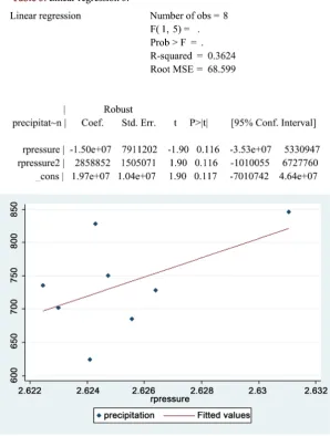
The result of regression analysis is Table 3.
The relationship between Precipitation and rpressure as Chart 5.
DOI: 10.4236/am.2017.810110 1522 Applied Mathematics
Table 3. Linear regression 3.
Chart 5. Precipitation model.
above, we could see that precipitation grows with rpressure in some condition. The model is:
2
precipitationk =197e+07 1.50− e+07 rpressure× k+2858852 rpressure× k (21)
4) Temperature model:
2 3
0 1 2 3
k k
t =d + × +d n d ×n +d ×n +u (10)
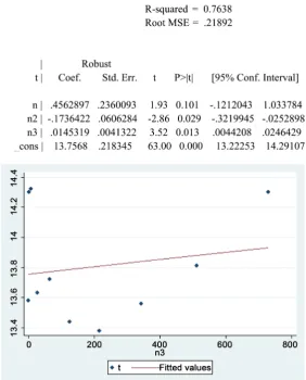
The result of regression analysis is as Table 4. The relationship between T and n is as Chart 6.
R-squared = 0.7638, which indicates this model explains the changes of tem-perature moderately, but there are some errors. Since test value of P by F is close to 0, the model is statistically significant in general, and is moderate fine. From the chart above, we could see that temperature grows with years in some condi-tion. The model is:
2 3
13.7568 0.4562897 0.1736422 0.0145319
k
DOI: 10.4236/am.2017.810110 1523 Applied Mathematics
Table 4. Linear regression 4.
Chart 6. Temperature model.
5) Forest area model
0 1 2 3
2 3
forest_areak =e + ×e rgdpk+ ×e rgdpk + ×e rgdpk+uk (11)
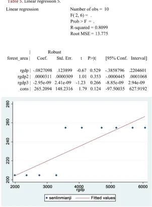
The result of regression analysis is as Table 5.
The relationship between Forest_area and rgdp as Chart 7.
R-squared = 0.8099, which indicates this model explains the changes between forest_area and rgdp well, but there are some inevitable errors as well. From the test result of F, the model is statistically significant in general, and is moderate fine. From the chart above, we could see that forest area grows with GDP per ca-pita in some condition. The model is:
3
2
forest_area 265.2094 0.0827098 0.0000311
2.95 09
k k
k
k
rgdp rgdp
e rgdp
= − × + ×
− − × (23)
6) Investment in water infrastructure model:
0 1
k k k
DOI: 10.4236/am.2017.810110 1524 Applied Mathematics
Table 5. Linear regression 5.
Chart 7.Forest model.
Using the same regression analysis in water supply model, we can get the re-sult of regression analysis is:
R-squared = 0.8099, which indicates this model explains the changes between investment and rgdp well, but there are some inevitable errors as well. From the test result of F, the model is statistically significant in general, and is moderate fine. From the chart above, we could see that investment grows with GDP per capita in some condition. The model is:
373.2892 0.431395
k k
i = − + ×rgdp (24)
7) Waste water discharge model:
2 3
0 1 2 3
rdischargek =g + ×g rgdpk+g ×rgdpk +g ×rgdpk+uk (13)
Using the same regression analysis in water supply model, we can get the re-sult of regression analysis is:
DOI: 10.4236/am.2017.810110 1525 Applied Mathematics R discharge and rgdp well, but there are some inevitable errors as well. From the test result of F, the model is statistically significant in general, and is moderate fine. From the chart above, we could see that R discharge grows with GDP per capita in some condition. The model is:
2
3
rdischarge 15.8245 0.0069993 2.31 07
6.48 11
k k k
k
rgdp e rgdp
e rgdp
= + × + − ×
− − × (25)
Using the same regression analysis in water supply model, we can get these results:
b) Water demand model
2
181.322 0.19625 2.31 06
k k k
d = + ×rgdp − e− ×rgdp (26)
c) GDP variation model:
677484 75.12275
k k
gdp = − + ×p (27)
d) Population model:
7876.886 7881.895
k k
r = − + ×sd (28)
All of these models are statistically significant in general, and the imitative ef-fect is fine.
3. Gansu Province with Teh Model
3.1. Water Scarcity Analysis by Using Model
After analyzing the water supply and demand in Shandong, we use the data in the last 20 years provided by China’s National Bureau of Statistics and use the same method to build a model of water supply and demand in Gansu:
a) Water supply model:
103.642 0.0572023 _ 0.0162697
k k k
s = + ×a w + ×i (29)
Available water quantity model in the nature:
_ _ 10 discharge
a w=z w− × (30)
Total water resource model in the nature:
_ k 173.4251 0.3355814 precipitationk 0.2315076 forest_areak
z w = − + × + × (31)
Precipitation model:
2
precipitationk =54e+05 1.23− e+04 rpressure× k+2245751 rpressure× k (32)
Temperature model:
2 3
8.4534 0.3545827 0.1369172 0.0267482
k
t = + × −n ×n + ×n (33)
Forest areas model:
2
3
forest_area 434.1398 0.0593192 0.0001563
4.26 07
k k k
k
rgdp rgdp
e rgdp
= − × + ×
− − × (34)
Investment in water infrastructure model:
174.3584 0.624367
k k
DOI: 10.4236/am.2017.810110 1526 Applied Mathematics Waste water discharge model:
2
3
rdischarge 4.8565 0.0256297 1.91 06
3.58 09
k k k
k
rgdp e rgdp
e rgdp
= + × + − ×
− − × (36)
Total waste water discharge:
discharge= ×p rdischarge (14)
b) Water demand model:
2
104.624 0.26645 3.51 07 k
k k
d = + ×rgdp − e− ×rgdp (37)
c) GDP variation model:
0 1
k k k
gdp =m +m ×p +u (16)
d) Population model:
2893.527 3012.847
k k
r = − + ×sd (38)
(
)
1 1
k k k
p =p− +r (18)
3.2. Water Situation in 15 Years
Time passes by 15 years from 2014, and we are in 2029. We use this model to forecast the water resources in Gansu, and here is the data as follows:
water resources in Gansu
2014 2029
a_w 132.4068 127.817
z_w 198.38 204.41
discharge 65,973.23 76,592.87
rdischarge 25.46 28.26
forest_area 507.45 511.27
gdp 6936.82 14,213.26
p 2591 2710
r 6.1 3
rgdp 26433 5244.7
i 608.13 1095
precipitation 420.2 463.3
t 8.7 10.95
d 120.57 129.94
s 120.57 119.54
s/d 1 0.92
3.3. The Impact of This Situation on the Residents
re-DOI: 10.4236/am.2017.810110 1527 Applied Mathematics source and investment in water infrastructure has increased to some extent, both the GDP per capita and waste water discharge have increased which leads to a unobvious increase and even a loss in water supply. The increase in GDP per ca-pita generates an obvious increase in water demand, and thus produces a scant water supply. Under this situation, on one hand the growth rate of population will fall, and reduce the water demand; on the other hand, government will in-crease the investment in water infrastructure, put a step forward on water con-servation and utilization and increase water supply to make S/D ≥ 1 to meet the needs of water.
4. Intervention Plan
Design an Intervention Plan
Our intervention plan is made up of four parts: A, B, C, D. Plan A: Alter the growing structure of crops
We should introduce a ban on large-scale reclamation, migration and high water-consuming plants in Hexi. Go a step further and reduce the planting area of intercropped wheat, corn and other common crops. Alleviate carrying capaci-ties of resources by developing the cultivation of low water-consuming and drought-enduring plants. Expanding the planting area of wine grape and high- quality beer barley to achieve the win-win outcome of water saving and income increasing.
Plan B: Plant trees, thus expanding the forest areas
Expand the planting areas of forest and grass, increase the vegetation cover rate and strengthen the water-holding capacity of land.
Plan C: Increase financial expenditure on science and technology studies Science and technology studies require the support from the financial policy. If science and technology studies receive more money, it will give a rise to the higher technological level of industrial production and irrigation, and thus re-ducing the industrial water consumption and agricultural water consumption.
Plan D: Increase financial expenditure on water infrastructure including water diversion and water conversion project
The Qinghai Lake is located closely to Gansu province, with which Gansu could conduct water conversion project that transforms the salt water in the lake into clean water. In addition, Gansu may construct water diversion project from nearby rivers. Both of the solutions will directly increase the water supply of Gansu. An increase of financial expenditure in water infrastructure will increase the amount of water diversion project, water harvesting project, water reserve project, water conversion project and pollution control project.
5. Conclusion
pre-DOI: 10.4236/am.2017.810110 1528 Applied Mathematics vious attempts to exacerbate or alleviate the problem of water scarcity and come up with several causes for water scarcity. With the help of the model, China’s Government can promote such effective solutions for water scarcity to other provinces, which will bring some changes for the citizens living there.
References
[1] Deng, H.P. (2001) The Influence of Climate and Land Use Change on Hydrology and Water Resources Research. Advance in Earth Sciences, No. 6.
[2] Li, Y., Zhang, J.D. and Luo, P. (2013) Atmospheric Precipitation Estimation Model Research. Meteorological and Environmental Sciences, No. 5.
[3] Vapor Pressure Calculation Formula.
http://wenku.baidu.com/link?url=I81MqdnJxQAc8WMfHQB7YvIzBsJqRIUq93bqY 1NJNFeeRCRUAyH_b4nmye7uIghZ0b-gVsPZmvjoCl8DGhWAVKsvanSncTj3Ng-2MzetABC
[4] Shi, C.N. and Wang, L.Q. (2006) An Econometric Analysis on Relations Between the Growth-Declining of Forest Resources and Economic Growth. Forestry Eco-nomic, No. 11.
[5] Dong, M. and Lin, Y. (2007) Infrastructure Investment to GDP: Model, Relation-ships, and Conclusion. Journal of Inner Mongolia Finance and Economics College, No. 2.
[6] Yin, J., Wu, Z.N. and Hu, C.H. (2007) Forecasting Model of Domestic Water De-mand Related to GDP. Journal of Water Resources & Water Engineering, No. 4. [7] Liu, J.Q., Zheng, T.G. and Song, T. (2009) Environmental Pollution and Economic