LexSemTm: A Semantic Dataset Based on All words Unsupervised Sense Distribution Learning

L

S

TM: A Semantic Dataset Based on All-words Unsupervised

Sense Distribution Learning

Andrew Bennett,♥_{Timothy Baldwin,}♥_{Jey Han Lau,}♥♦ Diana McCarthy,♣ _{and Francis Bond}♠

♥_{Dept of Computing and Information Systems, The University of Melbourne} ♦_{IBM Research}

♣ _{Dept of Theoretical and Applied Linguistics, University of Cambridge} ♠_{Linguistics and Multilingual Studies, Nanyang Technological University}

[email protected], [email protected], [email protected], [email protected], [email protected]

Abstract

There has recently been a lot of interest in unsupervised methods for learning sense distributions, particularly in applications where sense distinctions are needed. This paper analyses a state-of-the-art method for sense distribution learning, and op-timises it for application to the entire vocabulary of a given language. The optimised method is then used to pro-duce LEXSEMTM: a sense frequency and

semantic dataset of unprecedented size, spanning approximately 88% of polyse-mous, English simplex lemmas, which is released as a public resource to the com-munity. Finally, the quality of this data is investigated, and the LEXSEMTM sense

distributions are shown to be superior to those based on the WORDNET first sense

for lemmas missing from SEMCOR, and at

least on par with SEMCOR-based

distribu-tions otherwise.

1 Introduction

Word sense disambiguation (WSD), as well as more general problems involving word senses, have been of great interest to the NLP commu-nity for many years (for a detailed overview, see Agirre and Edmonds (2007) and Navigli (2009)). In particular, there has recently been a lot of work on unsupervised techniques for these problems. This includes unsupervised methods for perform-ing WSD (Postma et al., 2015; Chen et al., 2014; Boyd-Graber et al., 2007; Brody et al., 2006),

as well as complementary problems dealing with word senses (Jin et al., 2009; Lau et al., 2014).

One such application has been the automatic learning of sense distributions (McCarthy et al., 2004b; Lau et al., 2014). A sense distribution is a probability distribution over the senses of a given lemma. For example, if the nouncranehad two senses, bird and machine, then a hypo-thetical sense distribution could indicate that the noun is expected to take themachine meaning 60% of the time and the bird meaning 40% of the time in a representative corpus. Sense distribu-tions (or simple “first sense” information) are used widely in tasks including information extraction (Tandon et al., 2015), novel word sense detection (Lau et al., 2012; Lau et al., 2014), semi-automatic dictionary construction (Cook et al., 2013), lex-ical simplification (Biran et al., 2011), and tex-tual entailment (Shnarch et al., 2011). Automat-ically acquired sense distributions themselves are also used to improve unsupervised WSD, for ex-ample by providing a most frequent sense heuris-tic (McCarthy et al., 2004b; Jin et al., 2009) or by improving unsupervised usage sampling strate-gies (Agirre and Martinez, 2004). Furthermore, the improvement due to the most frequent sense heuristic has been particularly strong when used with domain-specific data (Koeling et al., 2005; Chan and Ng, 2006; Lau et al., 2014).

In addition, there is great scope to use these techniques to improve existing sense frequency re-sources, which are currently limited by the bottle-neck of requiring manual sense annotation. The most prominent example of such a resource is WORDNET (Fellbaum, 1998), where the sense

frequency data is based on SEMCOR (Miller et

al., 1993), a 220,000 word corpus that has been manually tagged with WORDNET senses. This

data is full of glaring irregularities due to its age and the limited size of the corpus; for example, the word pipe has its most frequent sense listed as tobacco pipe, whereas one might expect this to be tube carrying water or gas

in modern English (McCarthy et al., 2004a). This is likely due to the more common use of the

tobacco pipesense in mid-20th century liter-ature. The problem is particularly highlighted by the fact that out of the approximately 28,000 pol-ysemous simplex lemmas in WORDNET3.0,

ap-proximately 61% have no sense annotations at all, and less than half of the remaining lemmas have at least 5 sense annotations!

Unfortunately, there has been a lack of work investigating how to apply sense learning tech-niques at the scale of a full lexical resource such as WORDNET. Updating language-wide sense

frequency resources would require learning sense distributions over the entire vocabularies of lan-guages, which could be extremely computation-ally expensive. To make things worse, domain dif-ferences could require learning numerous distribu-tions per word. Despite this, though, we would not want to make these techniques scalable at the expense of sense distribution quality. Therefore, we would like to understand the tradeoff between the accuracy and computation time of these tech-niques, and optimise this tradeoff. This could be particularly critical in applying them in an indus-trial setting.

The current state-of-the-art technique for unsu-pervised sense distribution learning isHDP-WSI

(Lau et al., 2014). In order to address the above concerns, we provide a series of investigations ex-ploring how to best optimiseHDP-WSIfor large-scale application. We then use our optimised technique to produce LEXSEMTM,1 a semantic

and sense frequency dataset of unprecedented size, spanning the entire vocabulary of English. Finally, we use crowdsourced data to produce a new set of gold-standard sense distributions to accompany LEXSEMTM. We use these to investigate the

qual-ity of the sense frequency data in LEXSEMTM

with respect to SEMCOR.

1_{LEXSEMTM, as well as code for accessing LEXSEMTM} and reproducing our experiments is available via:

https://github.com/awbennett/LexSemTm

2 Background and Related Work

Given the difficulty and expense of obtaining large-scale and robust annotated data, unsuper-vised approaches to problems involving word learning and recognising word senses have long been studied in NLP. Perhaps the most fa-mous such problem is word sense disambiguation (WSD), for which many unsupervised solutions have been proposed. Some methods are very com-plex, performing WSD separately for each word usage using information such as word embeddings of surrounding words (Chen et al., 2014) or POS-tags (Lapata and Brew, 2004). On the other hand, most approaches make use of the difficult-to-beat most frequent sense (MFS) heuristic (McCarthy et al., 2007), which assigns each usage of a given word-type to its most frequent sense.

Given the popularity of the MFS heuristic, much of the past work on unsupervised tech-niques has focused on identifying the most fre-quent sense. The original method of this kind was proposed by McCarthy et al. (2004b), which re-lied on finding distributionally similar words to the target word, and comparing these to the can-didate senses. Most subsequent approaches have followed a similar approach, based on the words appearing nearby the target word across its to-ken usages. Boyd-Graber and Blei (2007) for-malise the method of McCarthy et al. (2004b) with a probabilistic model, while others take different approaches, such as adapting existing sense fre-quency data to specific domains (Chan and Ng, 2005; Chan and Ng, 2006), using coarse grained thesaurus-like sense inventories (Mohammad and Hirst, 2006), adapting information retrieval-based methods (Lapata and Keller, 2007), using ensem-ble learning (Brody et al., 2006), utilising the net-work structure of WORDNET(Boyd-Graber et al.,

2007), or making use of word embeddings (Bhin-gardive et al., 2015). Alternatively, Jin et al. (2009) focus on how best to use the MFS heuris-tic, by identifying when best to apply it, based on sense distribution entropy. Perhaps the most promising approach is that of Lau et al. (2014), due to its state-of-the art performance, and the fact that it can easily by applied to any language and any sense repository containing sense glosses.

explicitly described in terms of sense distribution learning (Chan and Ng, 2005; Chan and Ng, 2006; Lau et al., 2014), while the others implicitly learn sense distributions by calculating some kind of scores used to rank senses.

The state-of-the-art technique of Lau et al. (2014) that we are building upon involves performing unsupervised word sense induction (WSI), which itself is implemented using non-parametric HDP (Teh et al., 2006) topic mod-els, as detailed in Section 3. The WSI compo-nent, HDP-WSI, is based on the work of Lau et al. (2012), which at the time was state-of-the-art. Since then, however, other competitive WSI ap-proaches have been developed, involving complex structures such as multi-layer topic models (Chang et al., 2014), or complex word embedding based approaches (Neelakantan et al., 2014). We have not used these approaches in this work on account of their complexity and likely computational cost, however we believe they are worth future explo-ration. On the other hand, becauseHDP-WSIis implemented using topic models, it can be cus-tomised by replacing HDPwith newer, more ef-ficient topic modelling algorithms. Recent work has produced more advanced topic modelling ap-proaches, some of which are extensions of existing approaches using more advanced learning algo-rithms or expanded models (Buntine and Mishra, 2014), while others are more novel, involving vari-ations such as neural networks (Larochelle and Murray, 2011; Cao et al., 2015), or incorporat-ing distributional similarity of words (Xie et al., 2015). Of these approaches, we chose to experi-ment with that of Buntine and Mishra (2014) be-cause a working implementation was readily avail-able, it has previously shown very strong perfor-mance in terms of accuracy and speed, and it is similar to HDPand thus easy to incorporate into our work.

3 HDP-WSISense Learning

HDP-WSI (Lau et al., 2014) is a state-of-the-art unsupervised method for learning sense distri-butions, given a sense repository with per-sense glosses. It takes as input a collection of exam-ple usages of the target lemma2 _{and the glosses} 2_{Except where stated otherwise, a lemma usage includes} the sentence containing the lemma, and the two immediate neighbouring sentences (if available). It is assumed that each usage has been normalised via lemmatisation and stopword removal, and extra local-context tokens are added, as was

for each target sense, and produces a probability distribution over the target senses.

At the heart ofHDP-WSI isHDP (Teh et al., 2006), a nonparametric topic modelling technique. It is a generative probabilistic model and uses top-ics as a latent variable to allow statistical shar-ing between documents, providshar-ing a kind of soft-clustering mixture model. Each document is as-sumed to have a corresponding distribution over these topics, and each topic is assumed to have a corresponding distribution over words. Accord-ing to the model, each word for a given docu-ment is independently generated by first sampling a topic according to that document’s distribution over topics, and then sampling a word according to the topic’s distribution over words. Unlike older topic modelling methods such asLDA(Blei et al., 2003),HDPis nonparametric, meaning the num-ber of topics used by the model is automatically learnt, and does not need to be set as a hyper-parameter. In other words, the model automati-cally learns the “right” number of topics for each lemma.

HDP-WSI follows a two-step process: word sense induction (WSI), followed by topic–sense alignment. WSI is performed using HDP based on the earlier work of Lau et al. (2012): each us-age of the target lemma is treated as a document, andHDPtopic modelling is run on this document collection. This gives a variable number of learnt topics, which are the senses induced by WSI. A single topic is then assigned to each document,3

and a distribution over these topics is learnt using maximum likelihood estimation.

In the second step of HDP-WSI, we align the distribution over topics from WSI to the provided sense inventory. We first create a distribution over words for each sense, from the sense’s gloss.4

Then a prevalence score is calculated for each sense by taking a weighted sum of the similarity of that sense with every topic,5 _{weighting each}

similarity score by the topic’s probability. These prevalence scores are finally normalised to give a distribution over senses.

Despite state-of-the-art results withHDP-WSI

in past work (Lau et al., 2014), there are some

con-done by Lau et al. (2012).

3_{The topic with the maximum probability is assigned.} 4_{As with the lemma usages, the text is normalised via} lem-matisation and stopword removal. Then a distribution is cre-ated using maximum likelihood estimation.

cerns in applying it to large-scale learning. Most importantly, in order to make HDP nonparamet-ric, it relies on relatively inefficient MCMC sam-pling techniques, typically based on a hierarchi-cal Chinese Restaurant Process (“CRP”). On the other hand, recent work has provided very ef-ficient topic modelling techniques given a fixed number of topics. While in previous work it was assumed that performance benefits of HDP

over other techniques likeLDA were based on it learning the “right” number of topics (Lau et al., 2012; Lau et al., 2014), more recent work chal-lenges this assumption. Rather, it is suggested that it is more important for topic modelling to use high-performance learning algorithms so that top-ics are learnt in correct proportions, in which case “junk” topics can easily be ignored (Buntine and Mishra, 2014). In other words, it is likely that the previously-found performance advantage ofHDP

overLDA was actually due to properties of their respective Gibbs sampling algorithms.

Furthermore, in our experience using it for sense distribution learning, HDPseems to use a very consistent number of topics. In experiments we ran on theBNC6— the same dataset that Lau et

al. (2014) based their experiments on — the num-ber of topics was between 5 and 10 over 80% of the time, and over 99% of the time it was below 14. Because the number of topics is so consistent, it is likely we can safely use a fixed number with little risk that it will be too low.

In addition, there are some theoretical concerns with HDP. Firstly, it models topic and word al-locations using Dirichlet Processes (Teh et al., 2006). However, previous research has shown that phenomena such as word and sense frequen-cies follow power-law distributions according to Zipf’s law (Piantadosi, 2014), and thus are better modelled using Pitman-Yor Processes (Pitman and Yor, 1997). Another weakness is thatHDPdoes not model burstiness. This is a phenomenon where words that occur at least once in a given discourse are disproportionately more likely to occur several times, even compared with other discourses about the same topic (Church, 2000; Doyle and Elkan, 2009).

6_{The British National Corpus (Burnard, 1995), which is a} balanced corpus of English.

4 HCA-WSISense Learning

We now present and evaluate HCA-WSI, which is an alternative to HDP-WSI that addresses the above concerns. It follows the same process as HDP-WSI, except that the HDP topic mod-elling is replaced withHCA7_{(Buntine and Mishra,}

2014), a more advanced software suite for topic modelling.8 _{HCAis based on a similar}

probabilis-tic model to HDP, except for a few differences: (1) it only has a fixed number of topics; (2) it mod-els word frequencies using a more general Pitman-Yor Process; and (3) it incorporates an extra com-ponent to the model to model burstiness (each doc-ument can individually have an elevated probabil-ity for some words, regardless of its distribution over topics). The second and third of these dif-ferences directly answer our theoretical concerns about usingHDP.

The learning algorithm forHCAis called “table indicator sampling” (Chen et al., 2011), which is a collapsed Gibbs sampling algorithm. The over-all probabilistic model is interpreted as a hierar-chical CRP, and some extra latent variables called table indicators are added to the model, which en-code the decisions made about creating new tables during the CRP. The use of these latent variables allows for a very efficient collapsed Gibbs sam-pling process, which is found to converge more quickly than competing Gibbs sampling and vari-ational Bayes techniques. The convergence is also shown to be more accurate, with topic models of lower perplexity being produced given the same underlying stochastic model.

Compared to HDP, HCA has been shown to be orders of magnitude faster, with similar mem-ory overhead (Buntine and Mishra, 2014). There-fore, as long as the quality of the sense distribu-tions given byHCA-WSIare no worse than those fromHDP-WSI, it should be worthwhile switch-ing in terms of scalability. This massive reduction in computation time would be of particular benefit to our intended large-scale application.

4.1 Evaluation

We evaluate HCA-WSI in comparison to HDP-WSI using one of the sense tagged datasets of

7_{Version 0.61, obtained from:}

http://www.mloss.org/software/view/527

0 20 40 102

103

104

Number of Lemma Usages (1000’s)

Topic

Model

Training

Time

(s) Training Time forHDP-WSIvs.HCA-WSI

HDP-WSI HCA-WSI

Figure 1: Comparison of the time taken to train the topic models ofHDP-WSIandHCA-WSIfor each lemma in theBNCdataset. For each method,

one data point is plotted per lemma.

Koeling et al. (2005),9 _{which was also used by}

Lau et al. (2014). This dataset consists of 40 En-glish lemmas, and for each lemma it contains a set of usages of varying size from theBNCand a

gold-standard sense distribution that was created by hand-annotating a subset of the usages with WORDNET1.7 senses.

Using this dataset, we can calculate the qual-ity of a candidate sense distribution by calculat-ing its Jensen Shannon divergence (JSD) with re-spect to the corresponding gold-standard distribu-tion. JSD is a measure of dissimilarity between two probability distributions, so a lower JSD score means the distribution is more similar to the gold-standard, and is therefore assumed to be of higher quality.

Given our finding on topic counts in Section 3,

HCAwas run using a fixed number of 10 topics. Other settings were configured as recommended in theHCAdocumentation, or according to theHDP

settings used by Lau et al. (2014).10 _{This setup is}

also used in subsequent experiments, except where stated otherwise.

We proceeded by calculating the JSD scores of all lemmas in this dataset, using both methods. We performed a Wilcoxon signed-rank test on the two

9_{Koeling et al. (2005) also produced domain-specific} datasets for the same lemmas, however in order to keep our analysis focussed we only use the domain-neutral BNC

dataset.

10_{Initial values for concentration and discount parameters} for burstiness were set to 100 and 0.5 respectively, and the number of iterations was set to 300. Other hyperparameters were left with default values.

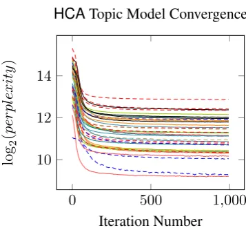
0 500 1,000 10

12 14

Iteration Number

log

2

(

per

pl

ex

ity

)

HCATopic Model Convergence

Figure 2: Convergence of log-perplexity of toic model forBNCdataset lemmas, usingHCA-WSI.

One line per lemma.

sequences of JSD scores, in order to test the hy-pothesis that switching toHCA-WSIhas a system-atic impact on sense distribution quality. We found that the mean JSD score forHDP-WSIwas 0.209

±0.116, slightly lower than the mean JSD score for HCA-WSI of 0.211 ± 0.117. However the two-sidedp-value from the test was 0.221, which is insignificant at any reasonable decision thresh-old.

In addition, we compared the time taken11 _to

run topic modelling for every lemma using both methods, the results of which are displayed in Fig-ure 1. These results show that the computation time ofHCA-WSIis consistently lower than that ofHDP-WSI, by over an order of magnitude.

We conclude thatHCA-WSIis far more compu-tationally efficient thanHDP-WSI, and there is no significant evidence that it gives worse sense dis-tributions. Therefore, HCA-WSIis used instead ofHDP-WSIfor the remainder of the paper.

5 Large-Scale Learning withHCA-WSI In order to apply HCA-WSI sense distribution learning on a language-wide scale, we need to understand how to optimise it to achieve a rea-sonable tradeoff between efficiency and sense dis-tribution quality. Most pertinently, we need to know how many lemma usages and iterations of Gibbs sampling are needed for high-quality re-sults, and whether this varies for different kinds of lemmas. To this end, we run experiments

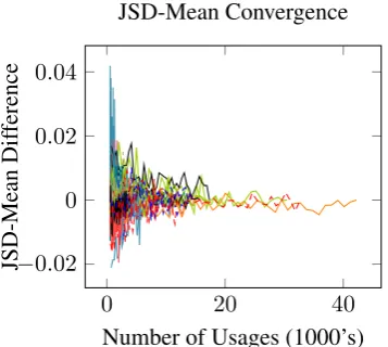
0 20 40 −0.02

0 0.02 0.04

Number of Usages (1000’s)

JSD-Mean

Dif

ference

JSD-Mean Convergence

Figure 3: Convergence of mean JSD score forBNC

dataset lemmas, usingHCA-WSI. One line plotted per lemma, one point per bin. For each data-point, the difference between mean JSD within that bin and within the final bin of the lemma is plotted.

ploring howHCA-WSIconverges over increasing numbers of lemma usages and topic model itera-tions. These experiments are all performed using theBNCdataset (see Section 4.1).

In order to explore the convergence of HCA-WSI over Gibbs sampling iterations, we trained

HCA topic models for each lemma in the BNC

dataset over a large number of iterations. The re-sults of this are displayed in Figure 2, which shows the convergence of log-perplexity for each lemma. We conclude that around 300 iterations of sam-pling appears to be sufficient for convergence in the vast majority of cases.

Next, we explored the convergence of HCA-WSIover lemma usages by subsampling from our training data. For each lemma in theBNCdataset,

we created a large number of sense distributions using random subsets of the lemma’s usages.12

Each distribution was generated by randomly se-lecting a number of usages between a minimum of 500 and the maximum available (uniformly), and randomly sampling that many usages without replacement. From these usages the sense distri-bution was created usingHCA-WSI, and its JSD score relative to the gold-standard was calculated (as in Section 4.1). Finally, the results for each lemma were partitioned into 40 bins of approxi-mately equal size, according to the number of us-ages sampled.

12_{Approximately 580 random sense distributions were} cre-ated per lemma.

The results of our subsampling experiment are plotted in Figure 3, which shows the convergence of mean JSD score for each lemma. We conclude from this that around 5,000–10,000 usages seem to be necessary for convergent results, and that this is fairly consistent across lemmas.13

6 LEXSEMTM Dataset

We now discuss the creation of the LEXSEMTM

(“Lexical Semantic Topic Models”) dataset, which contains trained topic models for the majority of simplex English lemmas. These can be aligned to any sense repository with glosses to produce sense distributions, or used directly in other ap-plications. In addition, the dataset contains distri-butions over WORDNET3.0 senses.

In order to produce domain-neutral sense dis-tributions reflecting usage in modern English, we sampled all lemma usages from English Wikipedia.14_{Our Wikipedia corpus was tokenised}

and POS-tagged using OpenNLP and lemmatised using Morpha (Minnen et al., 2001).

We trained topic models for every simplex lemma in WORDNET 3.0 with at least 20

us-ages in our processed Wikipedia corpus. This in-cluded lemmas for all POS (nouns, verbs, adjec-tives, and adverbs), and also nonpolysemous lem-mas. In Section 5, we concluded that approxi-mately 5,000–10,000 usages were needed for con-vergent results with theBNCdataset. On the other

hand, given that we are working on a different cor-pus and with a wider range of lemmas there is uncertainty in this number, so we conservatively sampled up to 40,000 usages per lemma, if avail-able.

These usages were sampled from the corpus by locating all sentences where either the surface or lemmatised forms of the sentence contained the target lemma, along with a matching POS-tag. Processing of lemma usages was done almost identically to Lau et al. (2014). However, because we found the usages contained substantially fewer tokens on average compared to the BNC dataset,

we included two sentences rather than one on ei-ther side of the target lemma location where pos-sible (giving 5 sentences in total), which gave a

13_{We also ran extensive experiments to test the impact of} training single topic models over multiple lemmas, using a wide variety of sampling methods, but found the impact to be neutral at best in terms of both the quality of the learned sense distributions and the overall computational cost.

better match in usage size.

Topic models were trained usingHCA, using al-most the same setup as described in Section 4.1. However, since some highly-polysemous lemmas may require a greater number of topics than the lemmas in theBNCdataset, we conservatively

in-creased the number of topics used from 10 to 20. We similarly increased the number of Gibbs sam-pling iterations from 300 to 1,000.15 _{Finally, for}

each polysemous lemma that we trained a topic model for, we also produced a sense distribu-tion over WORDNET3.0 senses, using the default

topic–sense alignment method discussed in Sec-tion 3.

In total, 62,721 lemmas were processed, and 8,801 of these had the desired number of at least 5,000 usages. Counting only polysemous lem-mas for which we also provide sense distribu-tions, 25,155 were processed in total, and 6,853 of these had at least 5,000 usages. This works out to approximately 88% coverage of polysemous WORDNET3.0 lemmas in total, or 24% coverage

with at least 5,000 usages (as compared to 39% coverage by lemmas in SEMCOR, or 17% with at

least 5 sense-tagged occurrences in SEMCOR).

7 Evaluation of LEXSEMTM against

SEMCOR

Our final major contribution is an analysis of how our LEXSEMTM sense distributions compare

with SEMCOR. We produce a new set of

gold-standard sense distributions for a diverse set of simplex English lemmas tagged with WORDNET

3.0 senses, created using crowdsourced annota-tions of English Wikipedia usages. We use these gold-standard distributions to investigate when LEXSEMTM should be used in place of SEM

-COR, and release them as a public resource, to

facilitate the evaluation of future work involving LEXSEMTM.

7.1 Gold-Standard Distributions

One of our goals in creating this dataset was to determine whether there is a SEMCORfrequency

cutoff,16 _{below which our LEXSEMTM}

distribu-tions are clearly more accurate than SEMCOR. In

order to have a diverse set of lemmas and be able

15_{These changes had a very minor impact on the} HCA-WSIevaluation results obtained in Section 4.1, with an aver-age increase in JSD of 0.001±0.004.

16_{The number of sense annotations in SEMCOR.}

to address this question, we partitioned the lem-mas in WORDNET 3.0 based on SEMCOR

fre-quency.

In order to keep analysis simple and consistent with previous investigations, we first filtered out multiword lemmas, nonpolysemous lemmas, and non-nouns.17 _{Next, since in Section 5 we decided}

that at least around 5,000 usages were needed for stable and converged sense distributions, we fil-tered out all lemmas without at least 5,000 usages in our English Wikipedia corpus. The remaining lemmas were then split into 5 groups of approx-imately equal size based on SEMCOR frequency.

The SEMCORfrequencies contained in each group

are summarised in Table 1.

From each of the SEMCOR frequency groups,

we randomly sampled 10 lemmas, giving 50 lem-mas in total. Then for each lemma, we randomly sampled 100 usages to be annotated from English Wikipedia. This was done in the same way as the sampling of lemma usages for LEXSEMTM (see

Section 6).

We obtained crowdsourced sense annotations for each lemma using Amazon Mechanical Turk (AMT: Callison-Burch and Dredze (2010)). The sentences for each lemma were split into 4 batches (25 sentences per batch). In addition, two con-trol sentences18_{were created for each lemma, and}

added to each corresponding batch. Each batch of 27 items was annotated separately by 10 an-notators. For each item to be annotated, annota-tors were provided with the sentence containing the lemma, the gloss for each sense as listed in WORDNET3.019and a list of hypernyms and

syn-onyms for each sense. Annotators were asked to assign each item to exactly one sense.

From these crowdsourced annotations, our gold-standard sense distributions were created us-ing MACE (Hovy et al., 2013), which is a general-purpose tool for inferring item labels from multi-annotator, multi-item tasks. It provides a Bayesian framework for modelling item annotations, mod-elling the individual biases of each annotator, and

17_{We chose to restrict our scope in this evaluation to nouns} because much of the prior work has also focussed on nouns, and these are the words we would expect others to care the most about disambiguating, since they are more often context bearing. Also, introducing other POS would require a greater quantity of expensive annotated data.

18_{These were created manually, to be as clear and} unam-biguous as possible.

supports semi-supervised training. MACE was run separately on the usage annotations of each lemma, with the control sentences included to guide training.

Gold-standard sense distributions were ob-tained from the output of MACE, which includes a list containing the mode label of each item. For each lemma, we removed the control sentence labels from this list, and constructed the gold-standard distribution from the remaining labels us-ing maximum likelihood estimation.

7.2 Evaluation of LEXSEMTM

We now use these gold-standard distributions to evaluate the sense distributions in LEXSEMTM

relative to SEMCOR. For each of the 50 lemmas

that we created gold-standard distributions for, we evaluate the corresponding LEXSEMTM

distribu-tion against the gold-standard. In addidistribu-tion, we cre-ate benchmark sense distributions for each lemma from SEMCORcounts using maximum likelihood

estimation,20 _{which we also evaluate against the}

gold-standards. Evaluation of sense distribution quality using gold-standard distributions is done by calculating JSD, as in Section 4.1.

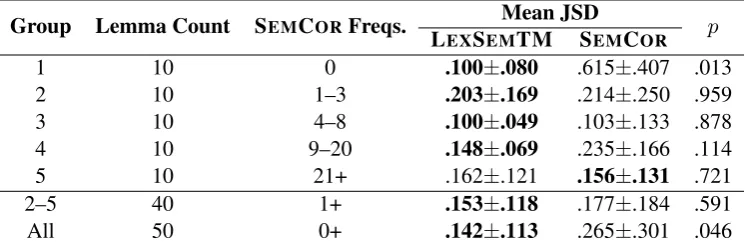
First, we performed this comparison of LEXSEMTM to SEMCOR JSD scores for all 50

lemmas at once. As in Section 4.1, we calcu-lated the JSD scores for every lemma using each method individually, and compared the difference in values pairwise for statistical significance us-ing a Wilcoxon signed-rank test. The results of this comparison are detailed in Table 1 (final row: Group = All), which shows that JSD is clearly lower for LEXSEMTM distributions compared to

SEMCOR, as would be hoped. This difference is

statistically significant atp <0.05.

We then performed the same comparison sepa-rately within each SEMCORfrequency group

(Ta-ble 1). First of all, we can see that LEXSEMTM

sense distributions strongly outperform SEMCOR

-based distributions in Group 1 (lemmas missing from SEMCOR). This is as would be expected,

since the SEMCOR-based distributions for this

group are based on which sense is listed first in WORDNET, which in the absence of SEMCOR

counts is arbitrary. On the other hand, in all other groups (lemmas in SEMCOR) the difference

be-tween LEXSEMTM and SEMCOR is not statisti-20_{For lemmas with no SEMCORannotations, we assign} one count to the first-listed sense in WORDNET3.0.

cally significant (p > 0.1in all cases). This still remains true when we pool together the results from these groups (second last row of Table 1: Group=2–5). While it appears that LEXSEMTM

may still be outperforming SEMCOR on average

over these groups (lower JSD on average), we do not have enough statistical power to be sure, given the high variance.

Returning to the initial question regarding a SEMCOR frequency cutoff, the only strong

con-clusion we can make is that LEXSEMTM is clearly

superior for lemmas missing from SEMCOR.

Al-though it appears that LEXSEMTM may

outper-form SEMCORfor lemmas with higher SEMCOR

frequencies, the variance in our results is too high to be sure of this, let alone define a frequency cutoff. However, given that LEXSEMTM sense

distributions never appear to be worse than SEM

-COR-based distributions, regardless of SEMCOR

frequency — and may actually be marginally su-perior — it seems reasonable to use our sense dis-tributions in general in place of SEMCOR.

We can contrast this result to the findings of McCarthy et al. (2007), who found that the au-tomatic first sense learning method of McCarthy et al. (2004b) outperformed SEMCOR for words

with SEMCOR frequency less than 5. However,

their analysis was based on the accuracy of the first sense heuristic, rather than the entire sense distribution, and they used very different datasets to us.21 _{Furthermore, their SEMCOR frequency}

cutoff result was only statistically significant for some variations of their method, and they evalu-ated over more lemmas22 _{meaning that statistical}

significance was easier to obtain. Given these rea-sons, their results likely do not contradict ours.

Given that LEXSEMTM contains sense

fre-quencies for 88% of polysemous simplex lemmas in WORDNET, compared to only 39% for SEM

-COR, the strong performance of our LEXSEMTM

sense distributions for lemmas missing from SEMCOR is extremely significant. Technically

these results are only relevant for lemmas where LEXSEMTM was trained on at least 5,000 us-21_{Their evaluation on the all words task from SENSEVAL} -2, which will have more occurrences of the more frequent words, whereas ours is a lexical sample with 100 instances of each word. However, our experiment has a larger dataset (50×100 = 5000instances, as opposed to 786 in total in the SENSEVAL-2 dataset) which makes it more reliable.

Group Lemma Count SEMCORFreqs. _L Mean JSD p EXSEMTM SEMCOR

1 10 0 .100±.080 .615±.407 .013

2 10 1–3 .203±.169 .214±.250 .959

3 10 4–8 .100±.049 .103±.133 .878

4 10 9–20 .148±.069 .235±.166 .114

5 10 21+ .162±.121 .156±.131 .721

2–5 40 1+ .153±.118 .177±.184 .591

All 50 0+ .142±.113 .265±.301 .046

Table 1: Sense distribution quality for gold-standard dataset lemmas, comparing LEXSEMTM results to

the SEMCORbenchmark.

ages, which reduces the coverage of LEXSEMTM

to 24%. However, even then this gives us sense frequencies for 1,602 polysemous lemmas miss-ing from SEMCOR, which accounts for over 5%

of polysemous simplex lemmas in WORDNET.

Furthermore, based on some additional ongoing analysis comparing LEXSEMTM distributions

di-rectly to SEMCOR-based distributions across all of

LEXSEMTM (not presented here), it appears the

decrease in sense distribution quality for lemmas trained on fewer than 5,000 usages is on average fairly small. This is corroborated by our results in Figure 3: we can observe for the lemmas in the

BNCdataset that when the number of usages was

reduced to 500, the mean change in JSD for each lemma was almost always less than 0.02 and never greater than 0.04, which is small compared to the difference between LEXSEMTM and SEMCORin

each SEMCOR frequency group. This strongly

suggests that our conclusions can be extended to lemmas with low LEXSEMTM frequency, though

more work is needed to confirm this.

8 Discussion and Future Work

The most immediate extension of our work would be to apply our sense learning method to a broader range of data. In particular, we intend to expand LEXSEMTM by applying HCA-WSI across the

vocabularies of languages other than English, and also to multiword lemmas. Another obvious ex-tension would be to further explore the alignment component ofHCA-WSI. We currently use a sim-ple approach, and we believe this process could be improved, e.g. by using word embeddings.

In addition, previous work by Lau et al. (2012) and Lau et al. (2014) also provided methods for detecting novel and unattested senses, us-ing the topic modellus-ing output from the WSI

step of HDP-WSI. These could be applied with LEXSEMTM— which contains this WSI output as

well as sense frequencies — to search for novel and unattested senses throughout the entire vocab-ulary of English. This could be used to expand ex-isting sense inventories with new senses, for exam-ple using the methodology of Cook et al. (2013). Given that LEXSEMTM also contains WSI output

for nonpolysemous WORDNET lemmas (37,566

in total), this could be lead to the discovery of many new polysemous lemmas.

In conclusion, we have created extensive re-sources for future work in NLP and related dis-ciplines. We have produced LEXSEMTM, which

was trained on English Wikipedia and spans ap-proximately 88% of polysemous English lemmas. This dataset contains sense distributions for the majority of polysemous lemmas in WORDNET

3.0. It also contains lemma topic models, for both polysemous and nonpolysemous lemmas, which provide rich semantic information about lemma usage, and can be re-aligned to sense invento-ries to produce new sense distributions at triv-ial cost. In addition, we have produced gold-standard distributions for a subset of the lemmas in LEXSEMTM, which we have used to demonstrate

that LEXSEMTM sense distributions are at least

on-par with those based on SEMCORfor lemmas

with a reasonable frequency in Wikipedia, and strongly superior for lemmas missing from SEM

-COR. Finally, we demonstrated that HCA topic

modelling is more efficient than HDP, providing guidance for others who wish to do large-scale un-supervised sense distribution learning.

Acknowledgements

References

Eneko Agirre and Philip Edmonds. 2007. Word

Sense Disambiguation: Algorithms and Applica-tions. Springer, Dordrecht, Netherlands.

Eneko Agirre and David Martinez. 2004. Unsuper-vised WSD based on automatically retrieved exam-ples: The importance of bias. InProceedings of the 2004 Conference on Empirical Methods in Natural Language Processing (EMNLP 2004), pages 25–32, Barcelona, Spain.

Sudha Bhingardive, Dhirendra Singh, V. Rudramurthy, Hanumant Redkar, and Pushpak Bhattacharyya. 2015. Unsupervised most frequent sense detection using word embeddings. InProceedings of the 2015 Conference of the North American Chapter of the Association for Computational Linguistics: Human Language Technologies, pages 1238–1243, Denver, USA.

Or Biran, Samuel Brody, and Noemie Elhadad. 2011. Putting it simply: a context-aware approach to lex-ical simplification. In Proceedings of the 49th An-nual Meeting of the Association for Computational Linguistics: Human Language Technologies, pages 496–501, Portland, USA.

David M Blei, Andrew Y Ng, and Michael I Jordan. 2003. Latent Dirichlet allocation. The Journal of Machine Learning Research, 3:993–1022.

Jordan Boyd-Graber and David Blei. 2007. PUTOP: Turning predominant senses into a topic model for word sense disambiguation. InProceedings of the 4th International Workshop on Semantic Evaluation (SemEval-2007), pages 277–281, Prague, Czech Re-public.

Jordan Boyd-Graber, David Blei, and Xiaojin Zhu. 2007. A topic model for word sense disambiguation. In Proceedings of the 2007 Joint Conference on Empirical Methods in Natural Language Process-ing and Computational Natural Language LearnProcess-ing, pages 1024–1033, Prague, Czech Republic.

Samuel Brody, Roberto Navigli, and Mirella Lapata. 2006. Ensemble methods for unsupervised WSD. InProceedings of the 21st International Conference on Computational Linguistics and the 44th annual meeting of the Association for Computational Lin-guistics, pages 97–104, Sydney, Australia.

Wray L Buntine and Swapnil Mishra. 2014. Ex-periments with non-parametric topic models. In

Proceedings of the 20th ACM SIGKDD Conference on Knowledge Discovery and Data Mining (KDD 2014), pages 881–890, New York City, USA.

Lou Burnard. 1995. User reference guide British Na-tional Corpus version 1.0. Technical report, Oxford University Computing Services, UK.

Chris Callison-Burch and Mark Dredze. 2010. Cre-ating speech and language data with Amazon’s Me-chanical Turk. In Proceedings of the North Amer-ican Chapter of the Association for Computational Linguistics Human Language Technologies 2009 (NAACL 2009): Workshop on Creating Speech and Text Language Data With Amazon’s Mechanical Turk, pages 1–12, Los Angeles, USA.

Ziqiang Cao, Sujian Li, Yang Liu, Wenjie Li, and Heng Ji. 2015. A novel neural topic model and its super-vised extension. In Proceedings of the 29th AAAI Conference on Artificial Intelligence, pages 2210– 2216, Austin, USA.

Yee Seng Chan and Hwee Tou Ng. 2005. Word sense disambiguation with distribution estimation. In Pro-ceedings of the 19th International Joint Conference on Artificial Intelligence, pages 1010–1015, Edin-burgh, UK.

Yee Seng Chan and Hwee Tou Ng. 2006. Estimat-ing class priors in domain adaptation for word sense disambiguation. InProceedings of the 21st Interna-tional Conference on ComputaInterna-tional Linguistics and 44th Annual Meeting of the Association for Com-putational Linguistics, pages 89–96, Sydney, Aus-tralia.

Baobao Chang, Wenzhe Pei, and Miaohong Chen.

2014. Inducing word sense with automatically

learned hidden concepts. In Proceedings of COL-ING 2014, the 25th International Conference on Computational Linguistics: Technical Papers, pages 355–364, Dublin, Ireland.

Changyou Chen, Lan Du, and Wray Buntine. 2011. Sampling table configurations for the hierarchical Poisson-Dirichlet process. In Machine Learning and Knowledge Discovery in Databases, volume 6912, pages 296–311. Springer.

Xinxiong Chen, Zhiyuan Liu, and Maosong Sun. 2014. A unified model for word sense represen-tation and disambiguation. In Proceedings of the 2014 Conference on Empirical Methods in Natural Language Processing (EMNLP), pages 1025–1035, Doha, Qatar.

Kenneth W. Church. 2000. Empirical estimates of adaptation: The chance of two noriegas is closer to p/2 thanp2_{. In Proceedings of the 18th}

Inter-national Conference on Computational Linguistics (COLING 2000), pages 180–186, Saarbr¨ucken, Ger-many.

Paul Cook, Jey Han Lau, Michael Rundell, Diana Mc-Carthy, and Timothy Baldwin. 2013. A lexico-graphic appraisal of an automatic approach for de-tecting new word senses. In Proceedings of eLex 2013, pages 49–65, Tallinn, Estonia.

Learning (ICML 2009), pages 281–288, Montreal, Canada.

Christiane Fellbaum. 1998. WordNet: An Electronic Lexical Database. MIT Press, Cambridge, USA.

Dirk Hovy, Taylor Berg-Kirkpatrick, Ashish Vaswani, and Eduard Hovy. 2013. Learning whom to trust with MACE. InProceedings of the 2013 Conference of the North American Chapter of the Association for Computational Linguistics: Human Language Technologies, pages 1120–1130, Atlanta, USA.

Peng Jin, Diana McCarthy, Rob Koeling, and John Car-roll. 2009. Estimating and exploiting the entropy of sense distributions. InProceedings of the North American Chapter of the Association for Computa-tional Linguistics Human Language Technologies (NAACL HLT 2009): Short Papers, pages 233–236, Boulder, USA.

Rob Koeling, Diana McCarthy, and John Carroll. 2005. Domain-specific sense distributions and pre-dominant sense acquisition. In Proceedings of the 2005 Conference on Empirical Methods in Natural Language Processing (EMNLP 2005), pages 419– 426, Vancouver, Canada.

Mirella Lapata and Chris Brew. 2004. Verb class disambiguation using informative priors. Computa-tional Linguistics, 30(1):45–73.

Mirella Lapata and Frank Keller. 2007. An informa-tion retrieval approach to sense ranking. InHuman Language Technologies 2007: The Conference of the North American Chapter of the Association for Computational Linguistics; Proceedings of the Main Conference, pages 348–355, Rochester, USA.

Hugo Larochelle and Iain Murray. 2011. The neural autoregressive distribution estimator. In Proceed-ings of the 14th International Conference on Ar-tificial Intelligence and Statistics (AISTATS 2011), pages 29–37, Fort Lauderdale, USA.

Jey Han Lau, Paul Cook, Diana McCarthy, David New-man, and Timothy Baldwin. 2012. Word sense in-duction for novel sense detection. In Proceedings of the 13th Conference of the EACL (EACL 2012), pages 591–601, Avignon, France.

Jey Han Lau, Paul Cook, Diana McCarthy, Spandana Gella, and Timothy Baldwin. 2014. Learning word sense distributions, detecting unattested senses and identifying novel senses using topic models. In Pro-ceedings of the 52nd Annual Meeting of the Asso-ciation for Computational Linguistics (ACL 2014), pages 259–270, Baltimore, USA.

Diana McCarthy, Rob Koeling, and Julie Weeds. 2004a. Ranking WordNet senses automatically. Technical Report 569, Department of Informatics, University of Sussex.

Diana McCarthy, Rob Koeling, Julie Weeds, and John Carroll. 2004b. Finding predominant word senses in untagged text. InProceedings of the 42nd An-nual Meeting of the Association for Computational Linguistics (ACL 2004), pages 280–287, Barcelona, Spain.

Diana McCarthy, Rob Koeling, Julie Weeds, and John Carroll. 2007. Unsupervised acquisition of pre-dominant word senses. Computational Linguistics, 33(4):553–590.

George A Miller, Claudia Leacock, and Randee Tengi. 1993. A semantic concordance. InProceedings of the ARPA Workshop on Human Language Technol-ogy, pages 303–308, Plainsboro, USA.

Guido Minnen, John Carroll, and Darren Pearce. 2001. Applied morphological processing of English. Nat-ural Language Engineering, 7(3):207–223.

Saif Mohammad and Graeme Hirst. 2006. Determin-ing word sense dominance usDetermin-ing a thesaurus. In

Proceedings of the 11th Conference of the EACL (EACL 2006), pages 121–128, Trento, Italy. Roberto Navigli. 2009. Word sense disambiguation: A

survey. ACM Computing Surveys, 41:1–69.

Arvind Neelakantan, Jeevan Shankar, Alexandre

Pas-sos, and Andrew McCallum. 2014. Efficient

non-parametric estimation of multiple embeddings per word in vector space. In Proceedings of the 2014 Conference on Empirical Methods in Natural Language Processing (EMNLP), pages 1059–1069, Doha, Qatar.

Steven T Piantadosi. 2014. Zipf’s word frequency law in natural language: A critical review and fu-ture directions. Psychonomic Bulletin & Review, 21(5):1112–1130.

Jim Pitman and Marc Yor. 1997. The two-parameter Poisson-Dirichlet distribution derived from a stable subordinator. The Annals of Probability, pages 855– 900.

Marten Postma, Ruben Izquierdo, and Piek Vossen. 2015. VUA-background : When to use background information to perform word sense disambiguation. InProceedings of the 9th International Workshop on Semantic Evaluation (SemEval-2015), pages 345– 349, Denver, USA, June.

Eyal Shnarch, Jacob Goldberger, and Ido Dagan. 2011. A probabilistic modeling framework for lexical en-tailment. InProceedings of the 49th Annual Meet-ing of the Association for Computational LMeet-inguis- Linguis-tics: Human Language Technologies, pages 558– 563, Portland, USA.

Yee Whye Teh, Michael I Jordan, Matthew J Beal, and David M Blei. 2006. Hierarchical Dirichlet pro-cesses. Journal of the American Statistical Associa-tion, 101:1566–1581.