Strategies for Training Large Vocabulary Neural Language Models

Strategies for Training Large Vocabulary Neural Language Models

Wenlin Chen David Grangier Michael Auli

Facebook, Menlo Park, CA

Abstract

Training neural network language mod-els over large vocabularies is computa-tionally costly compared to count-based models such as Kneser-Ney. We present a systematic comparison of neural strate-gies to represent and train large vocabular-ies, including softmax, hierarchical soft-max, target sampling, noise contrastive es-timation and self normalization. We ex-tend self normalization to be a proper esti-mator of likelihood and introduce an effi-cient variant of softmax. We evaluate each method on three popular benchmarks, ex-amining performance on rare words, the speed/accuracy trade-off and complemen-tarity to Kneser-Ney.

1 Introduction

Neural network language models (Bengio et al., 2003; Mikolov et al., 2010) have gained popular-ity for tasks such as automatic speech recognition (Arisoy et al., 2012) and statistical machine trans-lation (Schwenk et al., 2012; Vaswani et al., 2013; Baltescu and Blunsom, 2014). Similar models are also developed for translation (Le et al., 2012; De-vlin et al., 2014; Bahdanau et al., 2015), summa-rization (Chopra et al., 2015) and language gener-ation (Sordoni et al., 2015).

Language models assign a probability to a word given a context of preceding, and possibly sub-sequent, words. The model architecture deter-mines how the context is represented and there are several choices including recurrent neural net-works (Mikolov et al., 2010; Jozefowicz et al., 2016), or log-bilinear models (Mnih and Hinton, 2010). This paper does not focus on architec-ture or context representation but rather on how to efficiently deal with large output vocabularies, a problem common to all approaches to neural lan-guage modeling and related tasks (machine trans-lation, language generation). We therefore experi-ment with a classical feed-forward neural network model similar to Bengio et al. (2003).

Practical training speed for these models quickly decreases as the vocabulary grows. This is due to three combined factors: (i) model evaluation and gradient computation become more time con-suming, mainly due to the need of computing nor-malized probabilities over a large vocabulary; (ii) large vocabularies require more training data in order to observe enough instances of infrequent words which increases training times; (iii) a larger training set often allows for larger models which requires more training iterations.

This paper provides an overview of popular strategies to model large vocabularies for language modeling. This includes the classicalsoftmaxover all output classes,hierarchical softmaxwhich in-troduces latent variables, or clusters, to simplify normalization, target sampling which only con-siders a random subset of classes for normaliza-tion,noise contrastive estimation which discrim-inates between genuine data points and samples from a noise distribution, andinfrequent normal-ization, also referred as self-normalization, which computes the partition function at an infrequent rate. We also extend self-normalization to be a proper estimator of likelihood. Furthermore, we introducedifferentiated softmax, a novel variation of softmax which assigns more parameters, or ca-pacity, to frequent words and which we show to be faster and more accurate than softmax (§2).

Our comparison assumes a reasonable budget of one week for training models on a high end GPU (Nvidia K40). We evaluate on three benchmarks differing in the amount of training data and vocab-ulary size, that is Penn Treebank, Gigaword and the Billion Word benchmark (§3).

Our results show that conclusions drawn from small datasets do not always generalize to larger settings. For instance, hierarchical softmax is less accurate than softmax on the small vocabulary Penn Treebank task but performs best on the very large vocabulary Billion Word benchmark. This is because hierarchical softmax is the fastest method for training and can perform more training updates in the same period of time. Furthermore, our

sults with differentiated softmax demonstrate that assigning capacity where it has the most impact allows to train better models in our time budget (§4). Our analysis also shows clearly that tradi-tional Kneser-Ney models are competitive on rare words, contrary to the common belief that neural models are better on infrequent words (§5). 2 Modeling Large Vocabularies

We first introduce our model architecture with a classical softmax and then describe various other methods including a novel variation of softmax.

2.1 Softmax Neural Language Model

Our feed-forward neural network implements an n-gram language model, i.e., it is a parametric function estimating the probability of the next word wt _{given n − 1 previous context words,}

wt−1_{, . . . , w}t−n+1_{. Formally, we take as input a} sequence of discrete indexes representing then−1 previous words and output a vocabulary-sized vec-tor of probability estimates, i.e.,

f :{1, . . . , V}n−1→[0,1]V,

whereV is the vocabulary size. This function re-sults from the composition of simple differentiable functions orlayers.

Specifically,fcomposes an input mapping from discrete word indexes to continuous vectors, a suc-cession of linear operations followed by hyper-bolic tangent non-linearities, plus one final linear operation, followed by a softmax normalization.

The input layer maps each context word index to a continuousd0

0-dimensional vector. It relies on a matrixW0_∈RV×d0

0 to convert the input

x= [wt−1, . . . , wt−n+1]∈ {1, . . . , V}n−1

ton−1vectors of dimension d0

0. These vectors are concatenated into a single(n−1)×d0

0matrix,

h0 = [W_w0t−1;. . .;W_w0t−n+1]∈Rn−1×d00.

This state h0 _{is considered as ad0 = (n−1)×}

d0

0vector by the next layer. The subsequent states are computed throughklayers of linear mappings followed by hyperbolic tangents, i.e.

∀i= 1, . . . , k, hi _{= tanh(W}i_hi−1_+bi_)∈Rdi

where Wi _{∈ R}di×di−1, b ∈ Rdi are learn-able weights and biases and tanh denotes the component-wise hyperbolic tangent.

Finally, the last layer performs a linear operation followed by a softmax normalization, i.e.,

hk+1_=Wk+1_hk_+bk+1 _∈RV

and y= 1

Z exp(hk+1)∈[0,1]V (1)

whereZ =PV_j=1exp(hk_j+1)andexpdenotes the component-wise exponential. The network output

yis therefore a vocabulary-sized vector of proba-bility estimates. We use the standard cross-entropy loss with respect to the computed log probabilities

∂logyi

∂hk+1 j

=δij−yj

whereδij = 1ifi = j and0otherwise The gra-dient update therefore increases the score of the correct outputhk_i+1and decreases the score of all other outputshk_j+1forj6=i.

A downside of the classical softmax formulation is that it requires computation of the activations for

all output words, Eq. (1). The output layer with

V activations is much larger than any other layer in the network and its matrix multiplication domi-nates the complexity of the entire network.

2.2 Hierarchical Softmax

Hierarchical Softmax (HSM) organizes the out-put vocabulary into a tree where the leaves are the words and the intermediate nodes are latent variables, or classes (Morin and Bengio, 2005). The tree has potentially many levels and there is a unique path from the root to each word. The prob-ability of a word is the product of the probabilities of the latent variables along the path from the root to the leaf, including the probability of the leaf.

We follow Goodman (2001) and Mikolov et al. (2011b) and model a two-level tree. Given context

x, HSM predicts theclassof the next wordct_and the actual wordwt

p(wt|x) =p(ct|x)p(wt|ct, x) (2)

If the number of classes isO(√V)and classes are balanced, then we only need to computeO(2√V) outputs. In practice, this strategy results in weight matrices whose largest dimension is < 1,000, a setting for which GPU hardware is fast.

Wk+1 _hk

dA

dB

dC

|A|

|B|

|C| dA

dB

dC

Figure 1: Output weight matrix Wk+1 _and hid-den layerhk_{for differentiated softmax for} vocab-ulary partitions A, B, C with embedding dimen-sionsdA, dB, dC; non-shaded areas are zero.

contexts, relying on PCA (Lebret and Collobert, 2014). A full comparison of context-based clus-tering is beyond the scope of this work (Brown et al., 1992; Mikolov et al., 2013).

2.3 Differentiated Softmax

This section introduces a novel variation of soft-max that assigns a variable number of parameters to each word in the output layer. The weight ma-trix of the final layerWk+1 _{∈ R}dk×V stores

out-put embeddings of size dk for the V words the language model may predict: W₁k+1;. . .;W_Vk+1. Differentiated softmax (D-Softmax) varies the di-mension of the output embeddings dk across words depending on how much model capacity, or parameters, are deemed suitable for a given word. We assign more parameters to frequent words than to rare words since more training occurrences al-low for fitting more parameters.

We partition the output vocabulary based on word frequency and the words in each partition share the same embedding size. Partitioning the vocabulary in this way results in a sparse final weight matrix Wk+1 _{which arranges the} embed-dings of the output words in blocks, each block corresponding to a separate partition (Figure 1). The size of the final hidden layer hk _{is the sum} of the embedding sizes of the partitions. The fi-nal hidden layer is effectively a concatenation of separate features for each partition which are used to compute the dot product with the correspond-ing embeddcorrespond-ing type inWk+1_{. In practice, we} effi-ciently compute separate matrix-vector products, or in batched form, matrix-matrix products, for each partition inWk+1_andhk_.

Overall, differentiated softmax can lead to large speed-ups as well as accuracy gains since we can greatly reduce the complexity of computing the output layer. Most significantly, this strategy

speeds up both training and inference. This is in contrast to hierarchical softmax which is fast during training but requires even more effort than softmax for computing the most likely next word.

2.4 Target Sampling

Sampling-based methods approximate the soft-max normalization, Eq. (1), by summing over a sub-sample of impostor classes. This can signif-icantly speed-up each training iteration, depend-ing on the size of the impostor set. Target sam-pling builds upon the importance samsam-pling work of Bengio and Sen´ecal (2008). We follow Jean et al. (2014) who choose as impostors all positive examples in a mini-batch as well as a subset of the remaining words. This subset is sampled uni-formly and its size is chosen by validation.

2.5 Noise Contrastive Estimation

Noise contrastive estimation (NCE) is another sampling-based technique (Hyv¨arinen, 2010; Mnih and Teh, 2012; Chen et al., 2015). Contrary to target sampling, it does not maximize the train-ing data likelihood directly. Instead, it solves a two-class problem of distinguishing genuine data from noise samples. The training algorithm sam-ples a wordwgiven the preceding contextxfrom a mixture

p(w|x) = 1

k+ 1ptrain(w|x) +

k

k+ 1pnoise(w|x) where ptrain is the empirical distribution of the training set and pnoise is a known noise distri-bution which is typically a context-independent unigram distribution. The training algorithm fits the model pˆ(w|x) to recover whether a mixture sample came from the data or the noise distribu-tion, this amounts to minimizing the binary cross-entropy−y log ˆp(y= 1|w, x)−(1−y) log ˆp(y = 0|w, x) where y is a binary variable indicating where the current sample originates from

( ˆ

p(y= 1|w, x) = _pˆ(w|x)+pˆ(_kpw|_noisex) _(w|x) (data) ˆ

2.6 Infrequent Normalization

Devlin et al. (2014), followed by Andreas and Klein (2015), proposed to relax score nor-malization. Their strategy (here referred to as WeaknormSQ) associates unnormalized likeli-hood maximization with a penalty term that favors normalized predictions. This yields the following loss over the training setT

L(2)_α =− X

(w,x)∈T

s(w|x) +α X

(w,x)∈T

(logZ(x))2

where s(w|x) refers to the unnormalized score

of word w given context x and Z(x) =

P

wexp(s(w|x)) refers to the partition function for contextx. This strategy therefore pushes the log partition towards zero. For efficient training, the second term can be down-sampled

L(2) α,γ =−

X

(w,x)∈T

s(w|x)+α

γ

X

(w,x)∈Tγ

(logZ(x))2

whereTγ is the training set sampled at rateγ. A small rate implies computing the partition function only for a small fraction of the training data.

We extend this strategy to the case where the log partition term is not squared (Weaknorm), i.e.,

L(1)_α,γ =− X

(w,x)∈T

s(w|x) +α_γ X (w,x)∈Tγ

logZ(x)

Forα= 1, this loss is an unbiased estimator of the negative log-likelihood of the training dataL(2)₁ =

−P_(w,x)∈T s(w|x) + logZ(x). 3 Experimental Setup

Datasets We run experiments over three news datasets of different sizes: Penn Treebank (PTB), WMT11-lm (billionW) and English Gigaword, version 5 (gigaword). Penn Treebank (Marcus et al., 1993) is the smallest corpus with 1M tokens and we use a vocabulary size of10k (Mikolov et al., 2011a). The billion word benchmark (Chelba et al., 2013) comprises almost one billion tokens and a vocabulary of about 800k words1_.

Giga-word (Parker et al., 2011) is even larger with 5 bil-lion tokens and was previously used for language modeling (Heafield, 2011) but there is no standard train/test split or vocabulary for this set. We split according to time: training covers 1994–2009 and test covers 2010. The vocabulary comprises the 100k most frequent words in train. Table 1 sum-marizes the data statistics.

1_{T. Robinson versionhttp://tiny.cc/1billionLM.}

Dataset Train Test Vocab OOV

PTB 1M 0.08M 10k 5.8%

gigaword 4,631M 279M 100k 5.6%

billionW 799M 8.1M 793k 0.3%

Table 1: Dataset statistics. Number of tokens for train and test, vocabulary size, fraction of OOV.

Evaluation We measure perplexity on the test set. For PTB and billionW, we report results on a per sentence basis, i.e., models do not use context words across sentence boundaries and we score end-of-sentence markers. This is the standard set-ting for these benchmarks and allows comparison with other work. On gigaword, we use contexts across sentence boundaries and evaluation does not include end-of-sentence markers.

Our baseline is an interpolated Kneser-Ney (KN) model. We use KenLM (Heafield, 2011) to train 5-gram models without pruning. For neural mod-els, we train 11-gram models for gigaword and bil-lionW; for PTB we train a 6-gram model. The model parameters (weightsWi _{and biases b}i _for

i = 0, . . . , k + 1) are learned to maximize the training log-likelihood relying on stochastic gra-dient descent (SGD; LeCun et al.. 1998).

Validation Hyper-parameters are the number of layerskand the dimension of each layerdi,∀i = 0, . . . , k. We tune the following settings for each technique on the validation set: the number of clusters, the clustering technique for hierarchi-cal softmax, the number of frequency bands and their allocated capacity for differentiated softmax, the number of distractors for target sampling, the noise/data ratio for NCE, as well as the regular-ization rate and strength for infrequent normaliza-tion. Similarly, SGD parameters (learning rate and mini-batch size) are set to maximize validation likelihood. We also tune the dropout rate (Srivas-tava et al., 2014); dropout is employed after each tanh non-linearity.2

Training Time We train for 168 hours (one week) on the large datasets (billionW, gigaword) and 24 hours (one day) for Penn Treebank. All exper-iments are performed on the same hardware, a single K40 GPU. We select the hyper-parameters which yield the best validation perplexity after the allocated time and report the perplexity of the re-sulting model on the test set. This training time

2_{More parameter settings are available}

in an extended version of the paper at

is a trade-off between being able to do a compre-hensive exploration of the various settings for each method and good accuracy. The chosen training times are not long enough to observe over-fitting, i.e. validation performance is still improving – al-beit very slowly – at the end of the training session. As a general observation, even on the small PTB where 24 hours is rather long, we always found better results using the full training time, possibly increasing the dropout rate.

A concern may be that a fixing the training time favors models with better implementations. How-ever, all models are very similar and their core computations are always matrix/matrix products. Training differs mostly in the size and frequency of large matrix/matrix products. Matrix products rely on CuBLAS3_{, using torch}4_{. For the matrix}

sizes involved (>500×1,000), the time complex-ity of matrix product is linear in each dimension, both on CPU (Intel MKL5_{) and GPU (CuBLAS),}

with a10X speedup for GPU (Nvidia K40) com-pared to CPU (Intel Xeon E5-2680). Therefore, the speed trade-off applies to both CPU and GPU hardware, albeit with a different time scale.

4 Results

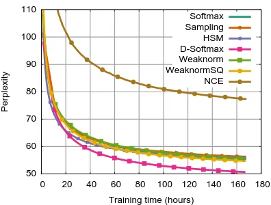
The test perplexities (Table 2) and validation learning curves (Figures 2, 3, and 4) show that the competitiveness of softmax diminishes with larger vocabularies. Softmax does well on the small vo-cabulary PTB but poorly on the large vovo-cabulary billionW corpus. Faster methods such as sam-pling, hierarchical softmax, and infrequent nor-malization (Weaknorm, WeaknormSQ) are much better in the large vocabulary setting of billionW.

D-Softmax is performing well on all sets and shows that assigning higher capacity where it ben-efits most results in better models. Target sam-pling performs worse than softmax on gigaword but better on billionW. Hierarchical softmax per-forms poorly on Penn Treebank which is in stark contrast to billionW where it does well. Noise contrastive estimation has good accuracy on bil-lionW, where speed is essential to achieving good accuracy.

Of all the methods, hierarchical softmax pro-cesses most training examples in a given time frame (Table 3). Our test time speed compari-son assumes that we would like to find the highest

3_{http://docs.nvidia.com/cuda/cublas/} 4_{http://torch.ch}

5_{https://software.intel.com/en-us/intel-mkl}

PTB gigaW billionW

KN 141.2 57.1 70.26

Softmax 123.8 56.5 108.3

D-Softmax 121.1 52.0 91.2

Sampling 124.2 57.6 101.0

HSM 138.2 57.1 85.2

NCE 143.1 78.4 104.7

Weaknorm 124.4 56.9 98.7

WeaknormSQ 122.1 56.1 94.9

KN+Softmax 108.5 43.6 59.4

KN+D-Softmax 107.0 42.0 56.3

KN+Sampling 109.4 43.8 58.1

KN+HSM 115.0 43.9 55.6

KN+NCE 114.6 49.0 58.8

KN+Weaknorm 109.2 43.8 58.1

KN+WeaknormSQ 108.8 43.8 57.7

Table 2: Test perplexity of individual models and interpolation with Kneser-Ney.

120 130 140 150 160 170 180 190

0 5 10 15 20

Perplexity

Training time (hours) Softmax Sampling HSM D-Softmax Weaknorm WeaknormSQ NCE

Figure 2: PTB validation learning curve.

scoring next word rather than rescoring an exist-ing strexist-ing. This scenario requires scorexist-ing all out-put words and D-Softmax can process nearly twice as many tokens per second than the other methods whose complexity is similar to softmax.

4.1 Softmax

Despite being our baseline, softmax ranks among the most accurate methods on PTB and it is sec-ond best on gigaword after D-Softmax (with Wea-knormSQ performing similarly). For billionW, the extremely large vocabulary makes softmax training too slow to compete with faster

alterna-6_{This perplexity is higher than reported in (Chelba et al.,}

50 60 70 80 90 100 110

0 20 40 60 80 100 120 140 160 180

Perplexity

Training time (hours) Softmax Sampling HSM D-Softmax Weaknorm WeaknormSQ NCE

Figure 3: Gigaword validation learning curve.

80 100 120 140 160 180

0 20 40 60 80 100 120 140 160 180

Perplexity

Training time (hours) Softmax Sampling HSM D-Softmax Weaknorm WeaknormSQ NCE

Figure 4: Billion Word validation learning curve.

train test

Softmax 510 510

D-Softmax 960 960

Sampling 1,060 510

HSM 12,650 510

NCE 4,520 510

Weaknorm 1,680 510

WeaknormSQ 2,870 510

Table 3: Training and test speed on billionW in to-kens per second for generation of the next word. Most techniques are identical to softmax at test time. HSM can be faster for rescoring.

50 60 70 80 90 100 110 120

0 10 20 30 40 50 60 70 80 90 100

Perplexity

Distractors per Sample (% of vocabulary) Sampling

Figure 5: Number of Distractors versus Perplexity for Target Sampling over Gigaword

tives. However, of all the methods softmax has the simplest implementation and it has no additional hyper-parameters compared to other methods.

4.2 Target Sampling

Figure 5 shows that target sampling is most accu-rate for distractor sets that amount to a large frac-tion of the vocabulary, i.e. > 30% on gigaword (billionW best setting>50% is even higher). Tar-get sampling is faster and performs more itera-tions than softmax in the same time. However, its perplexity reduction per iteration is less than soft-max. Overall, it is not much better than softsoft-max. A reason might be that sampling chooses distrac-tors independently from context and current model performance. This does not favor distractors the model incorrectly considers likely for the current context. These distractors would yield higher gra-dients that could update the model faster.

4.3 Hierarchical Softmax

Hierarchical softmax is very efficient for large vo-cabularies and it is the best method on billionW. On the other hand, HSM does poorly on small vo-cabularies as seen on PTB. We found that a good word clustering structure is crucial: when clusters gather words occurring in similar contexts, clus-ter likelihoods are easier to learn; when the clusclus-ter structure is uninformative, cluster likelihoods con-verge to the uniform distribution. This affects ac-curacy since words cannot have higher probability than their clusters, Eq. (2).

Our experiments organize words into a two level hierarchy and compare four clustering strate-gies on billionW and gigaword (§2.2). Random clustering shuffles the vocabulary and splits it into equally sized partitions. Frequency-based clustering first orders words based on their fre-quency and assigns words to clusters such that each cluster represents an equal share of the total frequency (Mikolov et al., 2011b). K-means runs the well-known clustering algorithm on Hellinger PCA word embeddings. Weighted k-means weights each word by its frequency.7

Random clusters perform worst (Table 4) fol-lowed by frequency-based clustering but k-means does best; weighted k-means performs similarly to its unweighted version. In earlier experiments, plain k-means performed very poorly since the most frequent cluster captured up to 40% of the

7_{The time to compute the clustering (multi-threaded word}

billionW gigaword

random 98.51 62,27

frequency-based 92.02 59.47

k-means 85.70 57.52

weighted k-means 85.24 57.09

Table 4: HSM with different clustering.

token occurrences. We then explicitly capped the frequency budget of each cluster to 10% which brought k-means on par with weighted k-means.

4.4 Differentiated Softmax

D-Softmax is the best technique on gigaword and second best on billionW after HSM. On PTB it ranks among the best techniques whose per-plexities cannot be reliably distinguished. The variable-capacity scheme of D-Softmax can as-sign large embeddings to frequent words, while keeping computational complexity manageable through small embeddings for rare words.

Unlike for hierarchical softmax, NCE or Wea-knorm, the computational advantage of Softmax is preserved at test time (Table 3). D-Softmax is the fastest technique at test time, while ranking among the most accurate methods. This speed advantage is due to the low dimensional rep-resentation of rare words which negatively affects the model accuracy on these words (Table 5).

4.5 Noise Contrastive Estimation

Although we report better perplexities than the original NCE paper on PTB (Mnih and Teh, 2012), we found NCE difficult to use for large vocabular-ies. In order to work in this setting where mod-els are larger, we had to dissociate the number of noise samples from the data to noise ratio in the modeled mixture. For instance, a data/noise ra-tio of1/50gives good performance in our exper-iments but estimating only 50 noise sample pos-teriors per data point is wasteful given the cost of network evaluation. Moreover,50samples do not allow frequent sampling of every word in a large vocabulary. Our setting considers more noise sam-ples and up-weights the data sample. This allows to set the data/noise ratio independently from the number of noise samples.

Overall, NCE results are better than softmax only for billionW, a setting for which softmax is very slow due to the very large vocabulary. Why does NCE perform so poorly? Figure 6 shows en-tropy on the validation set versus the NCE loss for several models. The results clearly show that

4 5 6 7 8 9 10

0.054 0.056 0.058 0.06 0.062 0.064

Ent

ropy

NCE Loss

Figure 6: Validation entropy versus NCE loss on gigaword for experiments differing only in learn-ing rates and initial weights. Each color corre-sponds to one experiment, with one point per hour.

ilar NCE loss values can result in very different validation entropy. Although NCE might make sense for other metrics such as BLEU (Baltescu and Blunsom, 2014), it is not among the best tech-niques for minimizing perplexity. Jozefowicz et al. (2016) recently drew similar conclusions.

4.6 Infrequent Normalization

Infrequent normalization (Weaknorm and Wea-knormSQ) performs better than softmax on bil-lionW and comparably to softmax on Penn Tree-bank and gigaword (Table 2). The speedup from skipping partition function computations is sub-stantial. For instance, WeaknormSQ on billionW evaluates the partition only on10% of the exam-ples. In one week, the model is evaluated and up-dated on 868M tokens (with 86.8M partition eval-uations) compared to 156M tokens for softmax.

1-4K 4-20K 20-40K 40-70K 70-100K

Kneser-Ney 3.48 7.85 9.76 10.76 11.57

Softmax 3.46 7.87 9.76 11.09 12.39

D-Softmax 3.35 7.79 10.13 12.22 12.69

Target sampling 3.51 7.62 9.51 10.81 12.06

HSM 3.49 7.86 9.38 10.30 11.24

NCE 3.74 8.48 10.60 12.06 13.37

Weaknorm 3.46 7.86 9.77 11.12 12.40

WeaknormSQ 3.46 7.79 9.67 10.98 12.32

Table 5: Test entropy on gigaword over subsets of the frequency ranked vocabulary; rank 1 is the most frequent word.

5 Analysis

5.1 Model Capacity

Training neural language models over large cor-pora highlights that training time, not training data, is the main factor limiting performance. The learning curves on gigaword and billionW indicate that most models are still making progress after one week. Training time has therefore to be taken into account when considering increasing capac-ity. Figure 7 shows validation perplexity versus the number of iterations for a week of training. This figure shows that a softmax model with1024 hidden units in the last layer could perform bet-ter than the 512-hidden unit model with a longer training horizon. However, in the allocated time, 512hidden units yield the best validation perfor-mance. D-softmax shows that it is possible to se-lectively increase capacity, i.e., to allocate more hidden units to the most frequent words at the ex-pense of rarer words. This captures most of the benefit of a larger softmax model while staying within a reasonable training budget.

5.2 Effect of Initialization

We consider initializing both the input word em-beddings and the output matrix from Hellinger PCA embeddings. Several alternative tech-niques for pre-training embeddings have been pro-posed (Mikolov et al., 2013; Lebret and Collobert, 2014; Pennington et al., 2014). Our experiment highlights the advantage of initialization and do not aim to compare embedding techniques.

Figure 8 shows that PCA is better than random for initializing both input and output word rep-resentations; initializing both from PCA is even better. We see that even after long training ses-sions, the initial conditions still impact the valida-tion perplexity. We observed this trend also with

80 100 120 140 160 180 200

0 50 100 150 200 250 300

Perplexity

Training tokens (millions) D-Softmax 1024x50K, 512x100K, 64x640K

D-Softmax 1024x50K, 256x740K Softmax 1024 Softmax 512

Figure 7: Validation perplexity per iteration on billionW for softmax and D-softmax. Softmax uses the same number of units for all words. The first D-Softmax experiment uses 1024 units for the 50K most frequent words, 512 for the next 100K, and 64 units for the rest; similarly for the second experiment. All experiments end after one week.

other strategies than softmax. After one week of training, HSM is the only method which can reach comparable accuracy to PCA initialization when the output matrix is randomly initialized.

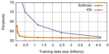
5.3 Training Set Size

Large training sets and a fixed training time in-troduce competition between slower models with more capacity and observing more training data. This trade-off only applies to iterative SGD op-timization and does not apply to classical count-based models, which visit the training set once and then solve training in closed form.

40 60 80 100 120 140 160 180 200

0 20 40 60 80 100 120 140 160 180

Perplexity

Training time (hours) Input: PCA, Output: PCA Input: PCA, Output: Random Input: Random, Output: PCA Input: Random, Output: Random

Figure 8: Effect of random initialization and with Hellinger PCA on gigaword for softmax.

55 60 65 70 75

0 0.5 1 1.5 2 2.5 3 3.5 4 4.5 5

Perplexity

Training data size (billions) Softmax

KN

Figure 9: Effect of training set size measured on test of gigaword for Softmax and Kneser-Ney.

500M tokens. In order to benefit from the full training set we would require a much higher train-ing budget, faster hardware, or parallelization.

Scaling training to large datasets can have a sig-nificant impact on perplexity, even when data from the distribution of interest is limited. As an illus-tration, we adapted a softmax model trained on bil-lionW to Penn Treebank and achieved a perplexity of96 - a far better result than with any model we trained from scratch on PTB (cf. Table 2).

5.4 Rare Words

How well do neural models perform on rare words? To answer this question, we computed entropy across word frequency bands for Kneser-Ney and neural models. Table 5 reports entropy for the4,000most frequent words, then the next most frequent 16,000 words, etc. For frequent words, neural models are on par or better than Kneser-Ney. For rare words, Kneser-Ney is very competitive. Although neural models might even-tually close this gap with much longer training, one should consider that Kneser-Ney trains on gi-gaword in only 8 hours on CPU which contrasts with 168 hours of training for neural models on high end GPUs. This result highlights the comple-mentarity of both approaches, as observed in our

interpolation experiments (Table 2).

For neural models, D-Softmax excels on fre-quent words but performs poorly on rare ones. This is because D-Softmax assigns more capacity to frequent words at the expense of rare words. Overall, hierarchical softmax is the best neural technique for rare words. HSM does more itera-tions than any other technique and so it can ob-serve every rare word more often.

6 Conclusions

This paper presents a comprehensive analysis of strategies to train neural language models with large vocabularies. This setting is very challeng-ing for neural networks as they need to compute the partition function over the entire vocabulary at each evaluation.

We compared classical softmax to hierarchical softmax, target sampling, noise contrastive esti-mation and infrequent normalization, commonly referred to as self-normalization. Furthermore, we extend infrequent normalization to be a proper es-timator of likelihood and we introduce differenti-ated softmax, a novel variant of softmax assigning less capacity to rare words to reduce computation. Our results show that methods which are ef-fective on small vocabularies are not necessarily equally so on large vocabularies. In our setting, target sampling and noise contrastive estimation failed to outperform the softmax baseline. Over-all, differentiated softmax and hierarchical soft-max are the best strategies for large vocabularies. Compared to classical Kneser-Ney models, neural models are better at modeling frequent words, but are less effective for rare words. A combination of the two is therefore very effective.

We conclude that there is a lot to explore in train-ing from a combination of normalized and unnor-malized objectives. An interesting future direc-tion is to combine complementary approaches, ei-ther through combined parameterization (e.g. hi-erarchical softmax with differentiated capacity per word) or through a curriculum (e.g. transitioning from target sampling to regular softmax as training progresses). Further promising areas are parallel training as well as better rare word modeling.

References

Ebru Arisoy, Tara N. Sainath, Brian Kingsbury, and Bhuvana Ramabhadran. 2012. Deep Neural Net-work Language Models. InNAACL-HLT Workshop on the Future of Language Modeling for HLT, pages 20–28, Stroudsburg, PA, USA. Association for Com-putational Linguistics.

Dzmitry Bahdanau, Kyunghyun Cho, and Yoshua Ben-gio. 2015. Neural machine translation by jointly learning to align and translate. InProc. of ICLR. As-sociation for Computational Linguistics, May.

Paul Baltescu and Phil Blunsom. 2014. Pragmatic neu-ral language modelling in machine translation. Tech-nical Report arXiv 1412.7119.

Yoshua Bengio and Jean-S´ebastien Sen´ecal. 2008. Adaptive importance sampling to accelerate train-ing of a neural probabilistic language model. IEEE Transactions on Neural Networks.

Yoshua Bengio, R´ejean Ducharme, Pascal Vincent, and Christian Jauvin. 2003. A Neural Probabilistic Lan-guage Model. Journal of Machine Learning Re-search, 3:1137–1155.

Peter F. Brown, Peter V. deSouza, Robert L. Mer-cer, Vincent J. Della Pietra, and Jenifer C. Lai. 1992. Class-based n-gram models of natural lan-guage. Computational Linguistics, 18(4):467–479, Dec.

Ciprian Chelba, Tom´aˇs Mikolov, Mike Schuster, Qi Ge, Thorsten Brants, Phillipp Koehn, and Tony Robin-son. 2013. One billion word benchmark for measur-ing progress in statistical language modelmeasur-ing. Tech-nical report, Google.

Xie Chen, Xunying Liu, MJF Gales, and PC Wood-land. 2015. Recurrent neural network language model training with noise contrastive estimation for speech recognition. InAcoustics, Speech and Signal Processing (ICASSP).

Sumit Chopra, Jason Weston, and Alexander M. Rush. 2015. Tuning as ranking. InProc. of EMNLP. Asso-ciation for Computational Linguistics, Sep.

Jacob Devlin, Rabih Zbib, Zhongqiang Huang, Thomas Lamar, Richard Schwartz, , and John Makhoul. 2014. Fast and Robust Neural Network Joint Models for Statistical Machine Translation. InProc. of ACL. Association for Computational Linguistics, June.

Joshua Goodman. 2001. Classes for Fast Maximum Entropy Training. InProc. of ICASSP.

Kenneth Heafield. 2011. KenLM: Faster and Smaller Language Model Queries. InWorkshop on Statistical Machine Translation, pages 187–197.

Michael Gutmann Aapo Hyv¨arinen. 2010. Noise-contrastive estimation: A new estimation principle for unnormalized statistical models. InProc. of AIS-TATS.

S´ebastien Jean, Kyunghyun Cho, Roland Memisevic, and Yoshua Bengio. 2014. On Using Very Large Target Vocabulary for Neural Machine Translation.

CoRR, abs/1412.2007.

Rafal Jozefowicz, Oriol Vinyals, Mike Schuster, Noam Shazeer, and Yonghui Wu. 2016. Exploring the lim-its of language modeling. Technical Report arXiv 1602.02410.

Hai-Son Le, Alexandre Allauzen, and Franc¸ois Yvon. 2012. Continuous Space Translation Models with Neural Networks. In Proc. of HLT-NAACL, pages 39–48, Montr´eal, Canada. Association for Computa-tional Linguistics.

Remi Lebret and Ronan Collobert. 2014. Word Em-beddings through Hellinger PCA. InProc. of EACL. Yann LeCun, Leon Bottou, Genevieve Orr, and Klaus-Robert Mueller. 1998. Efficient BackProp. In Genevieve Orr and Klaus-Robert Muller, editors,

Neural Networks: Tricks of the trade. Springer. Mitchell P. Marcus, Mary Ann Marcinkiewicz, and

Beatrice Santorini. 1993. Building a Large Anno-tated Corpus of English: The Penn Treebank. Com-putational Linguistics, 19(2):314–330, Jun.

Tom´aˇs Mikolov, Karafi´at Martin, Luk´aˇs Burget, Jan Cernock´y, and Sanjeev Khudanpur. 2010. Recurrent Neural Network based Language Model. InProc. of INTERSPEECH, pages 1045–1048.

Tom´aˇs Mikolov, Anoop Deoras, Stefan Kombrink, Lukas Burget, and Jan Honza Cernocky. 2011a. Empirical Evaluation and Combination of Advanced Language Modeling Techniques. InInterspeech. Tom´aˇs Mikolov, Stefan Kombrink, Luk´aˇs Burget, Jan

Cernock´y, and Sanjeev Khudanpur. 2011b. Exten-sions of Recurrent Neural Network Language Model. InProc. of ICASSP, pages 5528–5531.

Tom´aˇs Mikolov, Kai Chen, Greg Corrado, and Jeffrey Dean. 2013. Efficient Estimation of Word Represen-tations in Vector Space. CoRR, abs/1301.3781. Andriy Mnih and Geoffrey E. Hinton. 2010. A

Scal-able Hierarchical Distributed Language Model. In

Proc. of NIPS.

Andriy Mnih and Yee Whye Teh. 2012. A fast and simple algorithm for training neural probabilistic lan-guage models. InProc. of ICML.

Frederic Morin and Yoshua Bengio. 2005. Hierarchi-cal Probabilistic Neural Network Language Model. InProc. of AISTATS.

Robert Parker, David Graff, Junbo Kong, Ke Chen, and Kazuaki Maeda. 2011. English Gigaword Fifth Edi-tion. Technical report, Linguistic Data Consortium. Jeffrey Pennington, Richard Socher, and Christopher D

Holger Schwenk, Anthony Rousseau, and Mohammed Attik. 2012. Large, Pruned or Continuous Space Language Models on a GPU for Statistical Machine Translation. In NAACL-HLT Workshop on the Fu-ture of Language Modeling for HLT, pages 11–19. Association for Computational Linguistics.

Alessandro Sordoni, Michel Galley, Michael Auli, Chris Brockett, Yangfeng Ji, Margaret Mitchell, Jian-Yun Nie1, Jianfeng Gao, and Bill Dolan. 2015. A Neural Network Approach to Context-Sensitive Gen-eration of Conversational Responses. In Proc. of NAACL. Association for Computational Linguistics, May.

Nitish Srivastava, Geoffrey Hinton, Alex Krizhevsky, Ilya Sutskever, and Ruslan Salakhutdinov. 2014. Dropout: A simple way to prevent neural networks from overfitting. Journal of Machine Learning Re-search.