Munich Personal RePEc Archive
The mightier, the stingier: Firms’
market power, capital intensity, and the
labor share of income
Adrjan, Pawel
University of Oxford
13 January 2018
Online at
https://mpra.ub.uni-muenchen.de/83925/
The Mightier, the Stingier:
Firms’
Market Power, Capital Intensity,
and the Labor Share of Income
Pawel Adrjan*
Abstract
What determines the proportion of a firm’s income that workers receive as compensation? This
paper uses longitudinal firm data from a period of substantial labor share variation to
understand the firm-level determinants of the labor share of income—a question that has so far
only been addressed with country- and sector-level data. Firms with greater market power and
a higher ratio of capital to labor allocate a smaller proportion of their value added to workers.
These results suggest that firm-level drivers play a key role in the evolution of the aggregate
labor share, which have declined significantly since the 1970s.
JEL Codes: D33, E25, J24, J30
Keywords: Labor Share, Employee Compensation, Factor Income Distribution, Market Power, Capital Intensity
* Department of Economics, University of Oxford, Manor Road, Oxford OX1 3UQ, UK, pawel.adrjan@economics.ox.ac.uk
1
1. Introduction
The classic economic question of how rents are distributed among the factors of production
has recently returned to the fore, motivated by a substantial decline in labor’s share of national income in many of the world’s economies since the 1970s (Rodríguez and Jayadev,
2010; Elsby, Hobijn, and Şahin, 2013; Karabarbounis and Neiman, 2014; IMF, 2017). Figure
1 illustrates this decline for the G7 countries. From a starting point of approximately 70% in
1970, the aggregate labor share of income in this group of advanced economies has declined
by an average 2 percentage points per decade. This persistent downward trend contrasts with
the historical stylized fact of long-run stability of the labor share, which was prominently
noted by Keynes (1939) and Kaldor (1957) and has since become a standard assumption in
many micro- and macroeconomic models.
Several potential causes of the decline in the global labor share have been proposed.
One leading account is that technological change or declines in the price of capital relative to
labor have led firms to substitute capital for labor, thus decreasing the overall share of income
that accrues to the latter factor of production (Acemoglu, 2003; Bentolila and Saint-Paul,
2003; Karabarbounis and Neiman, 2014). Another is that deregulation or other drivers has
increased the market power of firms, raising the profit share of income at the expense of the
labor share (Blanchard and Giavazzi, 2003; Azmat, Manning, and Van Reenen, 2012; Barkai,
2016; Autor, Dorn, Katz, Patterson, and Van Reenen, 2017; De Loecker and Eeckhout,
2017). To date, however, both explanations have only been tested at the country and sector
level, even though the aggregate labor share is a result of the production decisions and
wage-setting processes occurring at individual, heterogeneous firms. In this paper, I propose a
methodology for calculating the labor share of value added at the firm level and use UK data
to show that the labor share varies significantly across firms, even within narrowly-defined
2
at individual firms. I find that firms with greater market power and a higher ratio of capital to
labor allocate a smaller proportion of their value added to workers. These results contribute to
a better understanding of the drivers of changes in aggregate factor income shares.
To motivate why the labor share might vary across and within firms, I describe a
simple model of a firm that employs capital and labor to produce a final good in an
imperfectly competitive product market. When the optimal combination of inputs is chosen to
maximize profits, the labor share is determined by the firm’s market power and the capital
intensity of production. Market power matters for the labor share because if a firm can set the
price of its product at a higher mark-up over cost, then a greater share of value added will go
to profits, at the expense of labor. Capital intensity matters too, because if a production
process is highly automated and requires little labor input, then under certain conditions, a
higher proportion of the firm's value added will be allocated towards compensating the
suppliers of capital. In the model, the exact nature of the relationship between capital
intensity and the labor share depends on the elasticity of substitution between labor and
capital and the nature of technical progress. Whether the labor share is higher or lower at
firms that employ more capital relative to labor is therefore an empirical question.
To test whether a firm’s market power and capital intensity impacts the labor share, I
use a large longitudinal dataset of firms in the United Kingdom covering the period from
2005 to 2012, during which the aggregate labor share experienced substantial fluctuations.
Thanks to mandatory filing requirements that affect nearly all incorporated businesses in the
UK, it is possible to calculate the labor share of value added for a wide universe of firms,
including small and medium enterprises, operating across a variety of sectors. Using the
model to motivate some potential drivers of this heterogeneity, I find an inverse relationship
between a firm’s labor share and its market power (measured by the market share), and
3
ratio). To account for potential endogeneity that may result, for instance, from a joint
response of variables to unobserved shocks, I estimate dynamic specifications of the model
using the Generalized Method of Moments (GMM). The finding that the labor share is
inversely related to the firm’s market power and capital intensity is robust to alternative
econometric methods, definitions of key variables, sample selection decisions, and empirical
specifications.
The results of this paper have several policy implications. As technological
developments and capital accumulation drive many economies to become more capital
intensive, my estimates suggest that labor’s share of aggregate income may continue to
decline. Similarly, the labor share might remain under pressure if economic activity becomes
increasingly concentrated in a smaller number of firms that wield greater market power at the
expense of the consumer, as some authors have suggested is the case (Barkai, 2016; Autor et
al., 2017; De Loecker and Eeckhout, 2017). Moreover, a declining labor share implies a
rising disconnect between average productivity and pay within the economy. This is because
the labor share of value added can be expressed as the ratio of average compensation to the
average product of labor. The link between productivity and pay matters greatly to
households, because wages and salaries represent by far the largest source of household
income in most developed countries. Understanding the determinants of firm-level labor
shares is therefore important for assessing the potential impact of future productivity gains or
losses on the earnings of the average household.
Does the finding that higher capital intensity of production lowers the labor share of
income mean that in the aggregate, capital and labor are substitutes? This result is consistent
with some strands of the factor share literature. For instance, Karabarbounis and Neiman
(2014) estimate an elasticity of substitution between capital and labor greater than 1 in their
4
relationship between the labor share and the capital-to-output ratio in sector-level data from
selected OECD countries. Piketty’s (2014) explanation of the global evolution of aggregate
income shares of capital and labor also relies on the high substitutability of these two factors
of production. On the other hand, an inverse relationship between capital intensity and the
labor share appears to be at odds with a large part of the literature that focuses specifically on
estimating the elasticity of substitution between capital and labor. The value of this elasticity
continues to be a matter of debate. While available estimates vary widely depending on the
methodology and context, often exceeding 1, many authors find lower values that imply a far
lesser degree of substitutability (see Chirinko, 2008, for a survey, and Knoblach, Rößler, and
Zwerschke, 2016, for a meta-analysis of US studies).
One possible reason for the divergent estimates of the aggregate elasticity of
substitution is that different classes of capital and labor are substitutable with one another to a
different extent. To understand whether this might drive my overall results, I carry out two
tests. First, I divide the sample into high-wage and low-wage firms, based on average
compensation per employee. I find that the negative effect of capital intensity on the labor
share is driven mainly by low-wage firms. Under the assumption that the average wage level
at a firm is a proxy for the average skill level of the workforce, these results imply that it is
mainly low-skilled labor that is substitutable for capital, rather than high-skilled labor.
Second, I consider the effects of tangible and intangible capital separately, based on the book
value of long-term tangible and intangible assets reported in firms’ financial statements.
Tangible assets are physical, fixed items such as machinery, buildings, and land, while
intangible assets represent nonphysical concepts such as patents, trademarks, and goodwill.
While it is often difficult to value intangible assets for accounting purposes, I find evidence
that an increase in intangible assets per employee has a positive effect on the labor share of
5
labor. The outcomes of both tests are consistent with intuition provided by the hypothesis of
capital-skill complementarity (Griliches, 1969). The paper thus contributes to bridging the
gap between the two opposing views on the potential impact of increases in capital intensity
on the labor share.
My results complement the macroeconomic literature on factor shares by focusing on
the determinants of the labor share at individual firms. Existing theoretical models of
aggregate labor share determination ascribe a leading role to factors that, in practice, vary
across narrowly-defined sectors and individual firms, such as the characteristics of production
technologies, relative quantities of capital and labor inputs, and the extent of monopoly
power in the product market (Bentolila and Saint-Paul, 2003; Azmat et al., 2012; Barkai,
2016; Autor et al., 2017; De Loecker and Eeckhout, 2017). The paper’s contributions to this
literature are to: a) construct firm-level measures of these variables using panel microdata, b)
show that the labor share varies substantially across firms, as well as within firms over time,
and c) exploit this variation to test hypotheses previously proposed in the context of a
representative firm and measured only using aggregate data. A firm-level focus is motivated
by the fact that in developed economies, most economic activity outside the public sector is
formally organized in firms. In the UK, for instance, the corporate sector represents
approximately 65% of aggregate gross value added, while private-sector employees account
for 75% of total employment (ONS, 2016). The sharing of income between labor and other
factors of production thus occurs primarily at this level. Understanding how the labor share at
individual firms is determined is therefore helpful for understanding the distribution of
aggregate national income.
This paper also extends a small body of recent research that has begun to use
firm-level data to analyze aggregate labor share trends. Growiec (2012) uses data on Polish firms
6
fluctuations. However, the author’s main focus is on short-run aggregate labor share
dynamics, whereas I assess the role of firm and market characteristics in determining the
level of the labor share at individual firms. Siegenthaler and Stucki (2015) exploit a survey of
4,000 Swiss manufacturing, construction and business service firms to estimate correlations
between the labor share and a firm’s use of computers, number of competitors, modern
organizational arrangements, participation in export markets, bargaining coverage, and the
share of female employees. In contrast to that paper, I use a large panel of firms operating in
all sectors of the business economy to test two leading hypothesized drivers of labor share
determination, capital intensity and market power. Moreover, I use methods designed to
address the potential endogeneity or simultaneity biases that may arise in estimating the
magnitude and direction of these relationships. Finally, Autor et al. (2017) use firm data from
several countries to construct measures of industry concentration and relate them to
sector-level labor share trends. The authors build a model, in which highly productive “superstar”
firms capture an increasing market share, leading to a fall in the aggregate labor share
through a reallocation of activity to such firms. Imposing a Cobb-Douglas production
function, which precludes any role for capital intensity, they document an empirical
association between rising industry concentration and declining labor shares within sectors.
My paper complements the analysis of Autor et al. (2017) in two main ways. First, it assesses
the relative effect of various determinants of the labor share at the level of individual firms,
rather than examining sectoral trends. Second, it allows both capital intensity and market
power to affect a firm’s labor share, allowing the magnitude of these two effects to be
compared. The role of capital intensity is particularly relevant, given the threat of
labor-to-capital substitution in many industrialized markets and its potential to put further downward
7
understand the underlying causes of the trends in the aggregate labor share, we should look
closely to firms, and the environment that they operate in, for answers.
The remainder of the paper is structured as follows. Section 2 discusses how to
measure the labor share of income at the firm level and documents the dispersion of labor
shares across firms and within firms over time. A simple model of the determinants of the
firm-level labor share is discussed in Section 3. Section 4 describes the data, and Section 5
outlines the empirical strategy. Section 6 presents the results and tests their robustness, while
Section 7 discusses the role of human capital and the firm’s labor market power in
determining the labor share. Section 8 concludes.
2. Measuring the labor share of income at the firm level
In this section, I discuss two types of contextual information relevant for the analysis of the
determinants of the labor share. First, I discuss how to measure the labor share of income
using data from firms’ financial reports in a way that mirrors the underlying economic
concept. Then, I show that firm-level labor shares are highly dispersed, even within
narrowly-defined sectors, which is inconsistent with the predictions of a fully competitive model. This
observation motivates the remainder of the paper, which explores the role of market power
and capital intensity in labor share setting.
The labor share is defined as the ratio of labor cost to some measure of income. In
standard formulations based on national accounts, the numerator typically includes both wage
and non-wage compensation of employees. In the denominator, income is usually measured
by aggregate gross value added.1
1 In the SNA 2008 national accounting framework, compensation of employees includes wages and salaries,
8
Labor Share =Labor CompensationIncome =Price of Value Added × Real Value AddedWage × Labor
A well-documented problem with this approach is that it does not account correctly for
self-employed individuals. While the output of the self-self-employed is part of national income, the
labor component of their remuneration is not captured in the compensation of employees.
This understates the labor share and affects cross-country comparisons (Gollin, 2002).2
In this paper, I focus on the firm-level labor share, using data on incorporated
businesses. One advantage over macroeconomic data is that focusing on firms and their
employees removes the confounding effects of self-employment on labor share estimates.
Although some self-employed individuals may in fact operate as incorporated businesses,
their impact on the data is mitigated by showing that the conclusions of this paper hold when
the smallest firms are excluded.
At the firm level, I define the labor share as the ratio of total employment expense to
gross value added. Like in the national accounts, employee compensation reported by
individual firms includes non-wage expenses, such as pension and health insurance expenses,
as well as social security taxes. I estimate firm-level gross value added as sales minus the cost
of intermediate inputs other than employee compensation (calculated from the financial
statements as earnings before interest, tax, depreciation, and amortization plus employee
compensation expense), adjusted for inventory growth:
Firm-Level Labor Share =Employee CompensationGross Value Added =Sales - Intermediate Inputs + ∆ InventoriesEmployee Compensation
Adding the change in inventories to the denominator aligns the firm-level measure of
value added with the corresponding economic concept of revenue-based output. Consider
2 Guerriero (2012) reviews a range of adjustments to the aggregate labor share proposed in the macroeconomic
9
what would happen if inventory changes were ignored. A firm that has produced goods in a
given period but has not yet sold them will have accounted for the full cost of labor, capital,
and other inputs used in production. Sales net of the cost of intermediate inputs will thus be
low, and the labor share will be overstated. Conversely, reported sales can reflect the running
down of inventories of final goods produced in earlier periods.
The adjustment for inventory changes is consistent with the way aggregate gross
value added is calculated in the national accounts (ONS, 2016). The existing literature on
firm-level labor shares has not incorporated this adjustment into its measures of gross value
added. However, year-to-year inventory changes at individual firms can be large. Excluding
them from the calculation of gross value added can affect the conclusions about the aggregate
evolution of the labor share. I demonstrate this in Section 4, in the context of the data sample.
When the numerator and denominator are divided by the number of employees, the
labor share becomes a ratio of the average wage to the average product of labor:3
Firm-Level Labor Share =
Employee Compensation Number of Employees
Gross Value Added Number of Employees
=Average Product of LaborAverage Compensation
The lower the labor share, the greater the gap between wages and average productivity. Firms
that have low labor shares thus undercompensate workers relative to the amount of output
they create. A declining labor share thus implies a “decoupling” of wages and productivity
and a shift in how the benefits of economic activity are shared with workers.
What does basic economic theory predict for the variation of labor shares across
firms? In a framework of competitive markets and free mobility of homogeneous input
factors, all profit-maximizing firms with identical, well-behaved production functions will
3 Average wages and productivity are expressed on a per-employee basis, as I do not have firm-level data on
10
choose the same technologically-efficient input allocation. In equilibrium, each factor will be
paid its marginal product, and the labor shares will be equal across firms. Nothing will be
gained by using firm-, rather than sector-level, data to analyze the determinants of the labor
share.
However, the data shows wide dispersion in firm labor shares. Table 1 presents
measures of between-firm and within-firm variation in the labor share and its components,
both in levels and in logs, derived from the random-effects model, 𝑥𝑖𝑡 = 𝛼 + 𝑢𝑖+ 𝜀𝑖𝑡 applied
to the pooled sample. Between-firm variation (𝜎𝑢/|𝑥̅|) is measured as the standard deviation
of the error term 𝑢𝑖 normalized by its mean, while within-firm variation (𝜎𝜀/|𝑥̅|) is measured
by the standard deviation of 𝜀𝑖𝑡, normalized by its mean. When the labor share is measured in
levels, between-firm variation is 0.40, and within-firm variation is 0.60, such that 31% of the
variance is due to differences across firms. The corresponding measures are 1.14 and 1.08
when the labor share is measured in logs, with 53% of the variance arising between firms.
The empirical strategy in this paper exploits both sources of variation.
The simplest framework that predicts no dispersion of the labor share also predicts no
dispersion in its individual components. Table 1 shows that both average compensation and
the average product of labor vary widely in the sample, and most of this variation is across
firms in the same industry. The fact that the ratio of these two variables is also dispersed
means that the numerator and denominator do not correlate perfectly. One way to see this is
to regress average compensation and the average product of labor and calculate 1 − 𝑅2 to
obtain the proportion of total variation in the former that is not explained by the latter.
Controlling for year and 4-digit sector fixed effects, this proportion is 54% when the
variables are measured in levels and 42% when the variables are measured in logs. The
11
3. Why might capital intensity and market power matter for the labor share?
This section outlines a simple model to illustrate why the labor share may differ across firms
within a given sector, even under the assumption that the production technologies are
identical. The aim is to motivate the empirical analysis that follows in an intuitive manner
before proceeding to a discussion of the data and the empirical strategy.4
To see why a firm’s labor share might be related to its market power and the capital
intensity of production, consider a profit-maximizing firm 𝑖 with the production function 𝑌𝑖 =
𝑌(𝐴𝑖𝐿𝑖, 𝐵𝑖𝐾𝑖), where 𝑌𝑖 is output, 𝐿𝑖 is labor, 𝐾𝑖 is capital, and 𝐴𝑖 and 𝐵𝑖 are labor- and
capital-augmenting productivity, respectively, which can vary across firms. Labor and capital
are supplied elastically at the wage 𝑤 and rental rate 𝑟, but the product market is imperfectly
competitive.5 From the first-order condition for labor, the labor share is
𝑠𝑖𝐿 ≡ 𝑤𝐿𝑃 𝑖 𝑖𝑌𝑖 = 𝜀𝑖
𝑌𝐿(1 + 1
𝜂𝑖) (1)
where 𝜀𝑖𝑌𝐿 =𝜕𝑌𝑖
𝜕𝐿𝑖 𝐿𝑖
𝑌𝑖 is the partial elasticity of output with respect to labor and 𝜂𝑖 = 𝜕𝑌𝑖 𝜕𝑃𝑖
𝑃𝑖 𝑌𝑖 is the
price elasticity of demand. The first term, 𝜀𝑖𝑌𝐿, is a function of the productivity parameters
and the labor and capital inputs. The firm’s labor share thus depends on the relative
productivity-augmented quantities of the factors employed in production. The sign of the
relationship between the labor share and the relative quantities of capital and labor inputs is
determined by the elasticity of substitution between capital and labor.6
4 For a discussion of similar predictions generated by general equilibrium models of monopolistic competition,
see Karabarbounis and Neiman (2014) and Barkai (2016).
5 Appendix C contains supporting derivations of key equations in the paper. The assumption of a perfectly
competitive labor market is relaxed in Section 7.
6 This point was first raised by Hicks (1932) and Robinson (1933). If the elasticity of substitution between
capital and labor is exactly 1 (like in the model of Autor et al. (2017), who assume a Cobb-Douglas production function), then the partial elasticity of output with respect to labor, 𝜀𝑖𝑌𝐿,will be independent of the firm’s capital-to-labor ratio. In that scenario, the empirical analysis that follows should find that capital per worker
does not matter for a firm’s labor share (which is not the case). Arpaia, Pérez, and Pichelmann (2009) develop a
12
If returns to scale in production are constant, then the first term of equation (1) can be
expressed more transparently as a function of the labor-to-capital ratio and the firm-specific
productivity parameters:
𝜀𝑖𝑌𝐿 ≡𝑌𝑌(𝐴𝐿(𝐴𝑖𝐿𝑖, 𝐵𝑖𝐾𝑖)
𝑖𝐿𝑖, 𝐵𝑖𝐾𝑖) 𝐿𝑖 = (
𝐴𝑖𝐿𝑖
𝐵𝑖𝐾𝑖)
𝑌𝐿(𝐴𝐵𝑖𝑖𝐾𝐿𝑖𝑖, 1)
𝑌 (𝐴𝑖𝐿𝑖
𝐵𝑖𝐾𝑖, 1)
= 𝑔 (𝐵𝐴𝑖𝐿𝑖
𝑖𝐾𝑖) (2)
where 𝑌𝐿 is the partial derivative of output with respect to labor. The empirical analysis that
follows will therefore test whether there is a relationship between the relative factor inputs
(measured as net tangible assets per employee) and the firm’s labor share, with the ratio of
productivity parameters absorbed by firm fixed effects.
The second term of equation (1) denotes the firm’s product market power and is
determined by the characteristics of demand. In the baseline specification of my empirical
analysis, I use the firm’s share of 4-digit sector sales to proxy for its product market power.
This is motivated by the observation that some models of imperfect competition predict a
direct relationship between the price elasticity of demand and firms’ market shares in
equilibrium. For example, consider a Cournot oligopoly with 𝑛 firms, each producing a
homogenous product with marginal cost 𝑐𝑖 and facing a linear inverse demand curve, 𝑃 =
𝑎 − 𝑏𝑄, where 𝑄 = ∑ 𝑞𝑖 𝑖 is total quantity produced. In equilibrium, firm 𝑖’s market share is
𝑠𝑖𝑀 ≡ 𝑞𝑖 ∑ 𝑞𝑖𝑖 =
𝑛+1 𝑛
𝑎−𝑐𝑖
𝑎−𝑐̅ − 1, where 𝑐̅ is the average marginal cost. The market share can be
expressed in terms of the elasticity of demand, 𝜂, as
𝑠𝑖𝑀 =(𝑛 + 1)(𝑎 − 𝑐𝑎 + 𝑛𝑐̅ 𝑖)(−𝜂) − 1 (3)
This illustrates a possible link between firms’ market shares and the price elasticity of
demand.7 The intuition is that when there are fewer firms in a sector, each firm’s market
7 In the empirical model, firm fixed effects absorb any firm-specific cost advantage, which will affect the
13
share is higher. Lower competition leads to greater monopoly power and a lower total
quantity produced, which corresponds to a more elastic part of the demand curve. This simple
model motivates the empirical analysis that follows, which uses longitudinal firm data to
estimate the firm-level determinants of the labor share.
4. Data
The main source of data for my analysis is the Financial Analysis Made Easy (FAME)
database supplied by Bureau van Dijk. It contains the financial filings of UK firms that
submit annual reports to Companies House, a government agency responsible for maintaining
the official company register. Virtually all companies in the UK, except the smallest ones, are
legally required to file an audited annual report. In 2015, the compliance rate with this
requirement was 99.1% (Companies House, 2015). Financial information follows
standardized accounting conventions. The audit requirement helps ensure that the data is of
high quality, partially mitigating potential concerns about reporting error. For these reasons,
FAME data is routinely used in research (e.g., Draca, Machin, and Van Reenen, 2011).
Thanks to strict reporting requirements, FAME contains information on a large
number of private and unlisted companies. Such companies represent the bulk of the total
firm count in the UK (and in most other countries), as well as a high proportion of aggregate
employment. The inclusion of small, private firms represents both an opportunity and a
challenge. On the one hand, it generates a more heterogeneous and representative sample of
firms than databases of listed companies, which exclude most small and medium enterprises.
On the other hand, many small firms are likely to be family businesses or self-employed
individuals operating as incorporated businesses. The labor share of such firms can easily be
between the (constant) price elasticity of demand and market shares as industry concentration changes.
14
mismeasured, since the labor and capital components of compensation are difficult to
disentangle in the case of business owners. Section 6 considers this issue explicitly and shows
that the results of this paper are robust to excluding the smallest firms from the sample.
The sample for analysis is defined by including all firms that report information on
labor compensation, sales, tangible assets, employment, and the line items needed to calculate
value added. This requirement makes the firms in the sample larger, on average, in terms of
sales and employment than the universe of UK firms. The financial sector is excluded due to
methodological differences in the calculation of value added. I also exclude sectors with a
substantial presence of non-market services (public administration, health, education, arts,
etc.), where value added can be difficult to measure. To avoid capturing foreign subsidiaries
of UK firms and their employees, I use unconsolidated financial accounts.
The result is a panel of 119,764 observations on 31,402 firms, covering the period
from 2005 to 2012. This period was characterized by substantial variation in the aggregate
labor share. Figure 2 shows that the aggregate labor share in the sample closely tracks the
corporate sector labor share calculated from the national accounts, and follows a similar
downward trend as the labor share in the UK economy and other G7 countries. (Notably,
while the Great Recession led the labor share to peak in 2009 as the value of output dropped
precipitously, it does not seem to have fundamentally altered the general downward trend
over this period.) The firms in the sample represent a substantial proportion of economic
activity generated by the UK non-financial corporate sector. In the last year of the sample
period, 2012, they generated total value added of £275bn, employed 5.8 million people, and
spent £167bn on employee compensation.
The sample includes firms of all sizes – from those employing a handful of
individuals to the largest businesses in the economy with hundreds of thousands of
15
variables used in the empirical analysis. Nominal values are converted to constant prices
using the GDP deflator. The median firm reports sales of £12 million and employment of 73.
It has a labor share of value added of 75%, £11,000 of tangible assets (net of accumulated
depreciation) per employee, and a share of 4-digit sector sales of less than 1%.
As mentioned in the discussion on measurement above, the year-to-year change in
inventories can be very large for an individual firm, substantially affecting firm-level
estimates of gross value added (and therefore the labor share). Inventory changes in the
sample range from a minimum of -£1.4bn to a maximum of +£1.8bn. To see the importance
of including inventory changes for the correct measurement of gross value added, consider
the impact of the financial crisis, which represented the largest shock to aggregate output
during the sample period. With the correct adjustment for inventory changes, aggregate
nominal GVA in the sample fell by 5.4% from 2008 to 2009. This falls squarely between the
4.3% decrease reported in the national accounts for “private non-financial corporations”
(ONS, 2016) and the 6.8% decrease reported in the aggregated results of the Annual Business
Survey of firms in the “non-financial business sector.”8 On the other hand, excluding the
inventory adjustment would have led incorrectly to an estimated nominal GVA increase in
the sample of 0.3%, contrary to the observed trend. This shows that correct measurement of
the labor share is important for drawing macroeconomic conclusions from firm-level data.
Table 2 also shows that, on average, a firm’s labor share declines as its capital
intensity rises. Firms with tangible assets per employee of less than £10,000 have a median
labor share of 81%. As the capital intensity rises across the sample, the average labor share
drops precipitously. For instance, firms with £50,000 to £100,000 of tangible assets per
worker have a median labor share of 66%, while firms with tangible assets per workers of
8 The Annual Business Survey is one of the sources used for calculating aggregate GVA in the national
16
£100,000 to £500,000 have a median labor share of 52%. In the right tail of firms with
tangible assets per worker of £500,000 or more, the median labor share is only 20%.
Similarly, the labor share declines with a firm’s market share. Firms with market
share within their 4-digit sector of less than 1% have a median labor share of 76%. The
average labor share declines gradually for firms observed with higher market shares. Like in
the case of capital intensity, the right tail of firms with market share of 20% or greater has the
lowest median labor share of 65%. Figure 3 illustrates this relationship visually. Both capital
intensity and market power thus appear to be potentially relevant determinants of the
firm-level labor share.
5. Empirical strategy
To assess whether the negative correlation between a firm’s labor share and its capital
intensity on one hand, and between the labor share and market share on the other, hold when
controlling for other confounding variables and addressing potential sources of endogeneity, I
estimate the following panel data model, based on log-linearized equation (1):
𝑠𝑖𝑡𝐿 = 𝛽 1(𝐾𝐿𝑖𝑡
𝑖𝑡) + 𝛽2𝑠𝑖𝑡 𝑀+ 𝜃
𝑗 + 𝜑𝑟+ 𝛿𝑡+ (𝑎𝑖+ 𝑣𝑖𝑡) (4)
𝑣𝑖𝑡 = 𝜌𝑣𝑖,𝑡−1+ 𝜀𝑖𝑡 (5)
𝜀𝑖𝑡 = 𝑀𝐴(0) (6)
where 𝑠𝑖𝑡𝐿 is the labor share at firm 𝑖 at time 𝑡; (𝐾𝑖𝑡
𝐿𝑖𝑡) is the capital-to-labor ratio and 𝑠𝑖𝑡
𝑀 is the
market share. Technology is permitted to vary across sectors 𝑗. The firm-specific labor share
is also allowed to be affected by factors specific to the region 𝑟 where the firm is located, and
by changes in the average labor share over time, denoted by the year fixed effects 𝛿𝑡. In the
main results that follow, the labor share is calculated as total compensation divided by value
17
of accumulated depreciation per employee, and product market power is estimated using the
firm’s share of 4-digit sector sales. I show later that the conclusions of this paper hold when
using alternative measures of these variables.
The labor share might also be determined by other sources of firm-level heterogeneity
besides market power and capital intensity. For instance, there can be permanent differences
in how value added is shared among labor and other factors of production, which may depend
on unobserved preferences of management, working conditions or other social and
organizational factors, or the relative size of the firm-specific productivity parameters 𝐴𝑖 and
𝐵𝑖. Such differences are captured by the time-invariant parameter 𝑎𝑖 in equation (4). In
addition, the labor share in any period may be affected by unobserved, firm-specific
productivity shocks. Following the standard approach used in the literature on estimating firm
production functions, I allow such shocks to be serially correlated. To derive a tractable
empirical specification, I assume that these shocks follow an AR(1) process given by
equation (5), where 𝜀𝑖𝑡 are random disturbances. This assumption is motivated by the
persistence of the firm-specific labor shares, market shares, and capital-to-labor ratios. It is
satisfactorily tested in the data, as discussed further below.
Two problems may arise in estimating equation (4) using ordinary least squares. One
is the potential correlation between the error term and the covariates. For instance, both the
capital-to-labor ratio and the labor share are likely to be jointly determined in response to
idiosyncratic shocks, 𝑣𝑖𝑡. In particular, firms may respond to shocks by adjusting the factor
input ratio. In other words, the firm's choice of capital intensity may be endogenous with
respect to 𝑣𝑖𝑡, such that 𝐸 [(𝐾𝑖𝑡
𝐿𝑖𝑡) 𝑣𝑖𝑡] ≠ 0. This will lead to biased results.
9
9 While the literature often assumes that adjusting the capital stock is costly and therefore capital responds to
18
A second problem is that time-invariant managerial or organizational characteristics,
captured by 𝜂𝑖, may be correlated with one or more regressors, such as the firm's choice of
factor inputs or market position. Reverse causality is also a concern. For instance, firms that
have a lower labor share than peers (𝑎𝑖 < 0) may find it easier and cheaper to fund increases
in their capital stock, thanks to their higher profits and the ability to offer a higher return on
capital. A low labor share might thus cause higher capital intensity, not the other way around.
If the shocks 𝑣𝑖𝑡 were serially uncorrelated (𝑣𝑖𝑡 = 𝜀𝑖𝑡), then the standard method for
dealing with these problems would consist of estimating equation (4) in differences to
eliminate the impact of permanent heterogeneity, 𝑎𝑖, and using instrumental variables to
address concerns about the correlation between the regressors and the error term. While
external instruments for firms’ input choices are typically difficult to find, lagged values of
the endogenous regressors themselves, dated 𝑡 − 2 or earlier, would be potentially valid
instruments, as they would be uncorrelated with the error term. In other words, the condition
𝐸[𝑥𝑖,𝑡−𝑠𝑣𝑖𝑡] = 0 would be satisfied for 𝑠 ≥ 2.
However, in practice, when the model is estimated using this procedure, the residuals
exhibit serial correlation. This casts doubt on the validity of a static model and suggests a
need to model serial correlation in the errors explicitly, like through equations (4) to (6). But
if the shocks are serially correlated, then the error term is a function of all past disturbances
𝜀𝑖1⋯ 𝜀𝑖𝑡. In this situation lagged values of the regressors are no longer valid instruments. A
model with firm fixed effects suffers from the same problem. Hence there is no consistent
way to estimate the static model.
Instead, the system (4)-(6) can be transformed into a dynamic model containing the
lagged labor share and lags of the regressors on the right-hand side. Solving (4) for 𝑣𝑖𝑡,
substituting into the autoregressive process (5), and first-differencing to remove the
19 ∆𝑠𝑖𝑡𝐿 = 𝜌∆𝑠𝑖,𝑡−1𝐿 + 𝜋1∆ (𝐾𝐿𝑖𝑡
𝑖𝑡) + 𝜋2∆ (
𝐾𝑖,𝑡−1
𝐿𝑖,𝑡−1) + 𝜋3∆𝑠𝑖𝑡 𝑀+ 𝜋
4∆𝑠𝑖,𝑡−1𝑀 + ∆𝜀𝑖𝑡 (7)
where 𝜋1 = 𝛽1, 𝜋2 = −𝜌𝛽1, 𝜋3 = 𝛽2, and 𝜋4 = −𝜌𝛽2. Following this transformation, lags
of any regressor 𝑥𝑖𝑡 dated 𝑡 − 2 or earlier are now potentially valid instruments for 𝑥𝑖𝑡 and
𝑥𝑖,𝑡−1, as 𝐸[𝑥𝑖,𝑡−𝑠𝜀𝑖𝑡] = 0 for 𝑠 ≥ 2. Similarly, 𝑠𝑖,𝑡−1𝐿 can be instrumented with lags of 𝑠𝑖𝑡𝐿
dated 𝑡 − 2 or earlier. The long-run relationship between capital intensity and the labor share
is then given by 𝜋1+𝜋2
1−𝜌 . Similarly, the long-run effect of market share on the labor share is
𝜋3+𝜋4
1−𝜌 . These parameters can be estimated consistently using two-stage least squares or the
Generalized Method of Moments (GMM).
Intuitively, a dynamic model with lags of the labor share, capital intensity, and market
share can be motivated by a delayed response of employment, investment, wages or sales to
shocks, especially when adjustments are costly. In the data, firms’ labor shares,
capital-to-labor ratios, and market shares are highly persistent over time. This observation is consistent
with either the presence of adjustment lags or serially correlated productivity shocks.
To estimate the coefficient vector (𝜌, 𝜋)', I use the System GMM estimator developed
by Arellano and Bover (1995) and Blundell and Bond (1998). In addition to using equation
(7) in first differences with lagged levels of the potentially endogenous variables as
instruments, System GMM exploits the unrestricted version of equation (4) in levels, with
lagged first-differences as instruments. This approach has two main advantages. First, it uses
more information by exploiting between-firm variation, which is a more important source of
overall variability in labor shares than within-firm variation. In the pooled sample, 79% of
variation in the log labor share is between—rather than within—firms. Second, System GMM
20
System GMM is the main approach used in the remainder of this paper.10 To avoid
concerns with overfitting (Roodman 2009), I limit the number of instruments to the lagged
levels dated 𝑡 − 2 and 𝑡 − 3 in the first-difference equation and lagged differences dated 𝑡 −
1 and 𝑡 − 2 in the levels equation, rather than using all past values. Appendix A contains a
detailed discussion of the assumptions required for the estimates to be consistent and
discusses how these assumptions have been tested in the data. The conclusion is that the
empirical model appears to be well-specified in responding to concerns about serial
correlation and potential endogeneity of the variables of interest.
6. Results: Firm-level determinants of the labor share of income
This section presents the findings on the relationship between market power, capital intensity,
and the labor share. It then explores the robustness of the results to alternative sample and
variable definitions, and empirical specifications.
Estimating the empirical model given by equation (4) gives a strong negative
relationship between the labor share and both market power and capital intensity. Table 3
presents the main results. The dependent variable in all columns is the log labor share,
defined as total compensation divided by value added. Column 1 regresses the log labor share
on capital intensity, measured as the log of net tangible assets per employee, and market
share, measured as the log of the firm’s share of 4-digit sector sales. Year fixed effects are
added to account for average trends in the labor share in the economy. The elasticity of the
labor share with respect to capital intensity is estimated to be -0.079. In other words, a
doubling of capital intensity is associated with a 7.9% reduction in the labor share.11 The
10 GMM estimation is carried out using the xtabond2 command in Stata, implemented by Roodman (2009), with
Windmeijer's (2005) finite-sample correction to the standard errors. I also report OLS results with a varying range of controls, and with and without firm fixed effects, to provide context for the GMM results.
11 Note that this is a percentage impact, not a percentage-point impact. The estimated elasticities are interpreted
21
estimated elasticity with respect to market share is much smaller in magnitude, at -0.009. A
doubling of the market share is thus associated with a 0.9% fall in the labor share. However,
both effects are highly statistically significant, with a p-value below 1%. Column 2 adds
sector fixed effects to control for sector-level differences in the labor share. The capital
intensity estimate falls slightly to -0.067, while the market share estimate increases
substantially in magnitude to -0.020. Both estimates remain highly statistically significant.
Column 3 adds region fixed effects to control for any geographic differences in labor share
setting that could be driven, for instance, by labor market conditions, but the impact on the
results is negligible.
OLS estimates thus highlight strong and significant correlations between firms’ labor
shares, market shares, and the capital intensity of production. However, as discussed earlier,
the coefficients will be biased in the presence of persistent shocks or unobserved
heterogeneity in how the labor share is determined at the firm level. Column 4 includes firm
fixed effects as one way to account for such unobserved heterogeneity. Firm-specific drivers
of the labor share may include things like within-sector product differentiation, differences in
production costs relative to competitors, or other aspects of the firm’s management and
organizational structure. The results reported in this column represent within-firm estimates
of the effects of an increase in capital intensity or market share on the labor share.
As discussed in Section 5, fixed-effects estimates may be biased if productivity
shocks are serially correlated. Column 5 of Table 3 therefore presents the results of GMM
estimation. This approach attempts to model this serial correlation explicitly while using
instrumental variable methods to address potential sources of endogeneity of the regressors.
The elasticity of the labor share with respect to capital intensity is -0.077, similar to the OLS
results, while the elasticity with respect to market share is -0.184, similar to the results with
22
between firms’ labor shares, market shares, and capital intensity. The Arellano and Bond
(1991) test for serial correlation does not highlight any second-order serial correlation in the
residuals (p-value 0.903), implying that there is no need to add more lags of the model
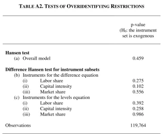
variables to ensure consistent estimation in the GMM framework. Moreover, the Hansen test
of overidentifying restrictions does not reject the null hypothesis of instrument exogeneity
(p-value 0.459). Together with the results of further tests in Appendix A, these diagnostics
suggest that the model is appropriate for the data and is estimated consistently.
The GMM estimates imply large effects of changes in a firm’s market power and
capital intensity on the labor share. For the average firm, a 1 percentage-point increase in
market share will lower the labor share by 9.5 percentage points, holding capital intensity of
production constant. If market share is held constant, on the other hand, then the same 9.5
percentage-point decline in the labor share would also arise if net tangible assets per
employee increased by approximately £59,000. One way to think about this amount is that it
is equivalent to 2 times the median employee compensation cost in the sample. Thus, net
investment equal to two years of labor costs would be expected to reduce the labor share of
income by almost 10 points, all else remaining constant.
An alternative way to assess the magnitude of the estimates in the context of the
sample is to consider how much market shares and capital intensities actually vary across
firms. Most firms observed in the data have low market shares and low capital intensity, but
the distributions of both variables are highly skewed to the right, with a large standard
deviation relative to the mean. A one standard deviation rise in market share (4.4 percentage
points) is estimated to lower the labor share of the average firm by 42.1 percentage points. A
move of this size implies almost a tripling of the share of sector sales by the average firm. On
the other hand, a one standard deviation rise in net tangible assets per employee (£102,000)
23
effect is relatively smaller than that for market share, given the smaller absolute size of the
estimated elasticity of the labor share with respect to capital intensity.
The finding that higher capital intensity lowers the labor share is consistent with the
claims of Karabarbounis and Neiman (2014) and Piketty (2014), who explain the trends in
aggregate factor income shares through an elasticity of substitution between capital and labor
greater than one. However, as mentioned above, the degree to which capital and labor are
substitutable is a matter of ongoing debate.
One reason why the conclusions about the substitutability of capital and labor may
vary is that different types of capital assets and workers may substitute or complement each
other differently. I therefore probe the relationship between capital intensity and the labor
share in three ways. First, to determine whether the effect of capital intensity differs
according to the skill level of a firm’s workforce, I split the sample into low-wage and
high-wage firms. I define high-high-wage firms as those that, on average, are in the top half of the
annual distribution of total compensation per employee during their presence in the sample.
Given that firms’ financial reports contain no information about the characteristics of
individual workers, I take the average wage level to be a proxy for the skill level of the
employees.12 This helps me judge whether the conclusions about the degree of substitutability
between capital and labor vary depending on the type of workforce that firms employ.
Second, to determine whether labor is equally substitutable with different classes of capital, I
add intangible capital intensity, defined as the log of the book value of intangible assets per
employee, as a regressor. Third, I combine the two approaches above to determine how the
two types of workforces and two types of capital interact.
12 Table B2 in the Appendix shows that the sample firms classified as high-wage are more concentrated in
24
It turns out that the aggregate results on capital intensity are driven mainly by
low-wage firms, suggesting that a low-skilled workforce is more substitutable with capital than a
high-skilled workforce. Moreover, higher intangible capital intensity leads to a higher labor
share, but only in the case of firms with a high-skilled workforce. These results are presented
in Table 4. In column 1, tangible capital intensity is interacted with an indicator for whether
the firm is a high-wage firm. The estimated elasticity for low-wage firms is -0.126, larger in
magnitude than the aggregate estimate and highly significant. While the estimate for
high-wage firms is also negative at -0.034, it is smaller and not statistically significant. Therefore,
to the extent that a firm’s average wage level can proxy for the average skills of its
workforce, these results suggest that high-skilled workers are much less substitutable with
(tangible) capital than low-skilled workers. Next, column 2 shows that the estimated elasticity
of the labor share with respect to intangible capital intensity is 0.023 and marginally
insignificant at a 10% level. Column 3 shows that the estimate on intangible capital intensity
is driven entirely by high-wage firms. On the assumption that firms with high average wages
have a workforce with high average skills, this suggests that high-skilled workers are less
substitutable with intangible capital than low-skilled workers, while low-skilled workers are
more substitutable with tangible capital than high-skilled workers.
How robust are the results to the way the sample has been defined and to the details of
the empirical specification? This is tested in Table 5 by modifying the baseline GMM
specification in several ways. Columns 1 to 3 address potential concerns with sample
selection. One such concern is that the universe of incorporated firms that submit financial
reports to Companies House may include self-employed individuals. I therefore check
whether the estimated coefficients change when firms that are never observed with more than
one employees are excluded from the sample. Column 1 reports these results. The estimated
25
share, both significant at a 1% level and similar in magnitude to those obtained from the full
sample. The main reason is that the smallest firms are typically not required to supply fully
detailed financials, and therefore few of them make it into the main sample. Next, column 2
focuses on firms observed in each year of the sample period. These tend to be larger and
more established firms. This sub-sample is therefore more likely to satisfy the assumptions of
System GMM (see Appendix A for a discussion). Again, the results are similar to the
baseline model in column 5 of Table 3. The estimated effect of capital intensity on the labor
share is larger in magnitude at -0.095, but the difference is not significant, while the
estimated effect of the market share is almost identical at -0.182. Finally, column 3 tests the
impact of outliers by estimating the model using unwinsorized variables. While this adds
some noise to the data and the coefficient estimates shift slightly, the results remain very
similar to those in the baseline GMM model.
Columns (4) to (8) explore different functional forms. Column 4 presents estimates in
levels, rather than logs. In column 5 only capital intensity is in logs, while the labor share and
market share are in levels. In column 6, only the labor share is in levels. Columns 7 and 8 add
squared terms to the log-log model, with the square of both capital intensity and market share
included in column 7 and only the square of market share in column 8. The market share
remains negative and statistically significant across these specifications, with differing
magnitudes in columns 4 to 6 reflecting the fact that the interpretation of the coefficient
changes depending on whether the variables are expressed in logs or in levels. Similarly,
market share enters negatively and significantly when its square is included in the log-log
model, with an elasticity at the mean similar to that obtained in the linear model. Capital
intensity, on the other hand, is less robust to changes in the model specification.
Finally, Table 6 shows that the overall conclusions are robust to several alternative
26
replaces the dependent variable with the wage share of value added, excluding non-wage
benefits such as pensions and social security taxes from the numerator. The estimated
elasticities with respect to capital intensity and market share of -0.070 and -0.201,
respectively, differ little from those in the baseline specification. This suggests that the
effects on the labor share operate mainly through wages, and not through other forms of
compensation. Column 2 redefines capital intensity as total assets per employee to account
for the potential role of intangible inputs in firms’ production functions and thus in
determining a firm’s labor share. The elasticity estimates of -0.070 and -0.188 remain in the
similar range as before. While this could be interpreted to mean that intangible assets are not
an important input for the average firm, it could also reflect the difficulty associated with
measuring intangible assets on the balance sheets of firms. Reassuringly, however, using total
assets as a measure of capital does not change the conclusions.
Next, columns 3 to 6 test alternative measures of market power. A firm’s share of
4-digit sector value added, rather than sales, is used in column 3, and the share of sales within
the sector and NUTS3 region (approximately equivalent to a county) is used in column 4.
Column 5 then repeats the specification from column 4 while restricting the sample to
non-tradable sectors, as defined by Mano and Castillo (2015). Finally, column 6 estimates market
power by the log of the ratio of value added to sales, as a proxy for the markup. Since this
variable is highly correlated with the denominator of the labor share, it is instrumented with
lags dated 𝑡 − 3 and 𝑡 − 4 for the equation in levels and 𝑡 − 4 and 𝑡 − 5 for the equation in
first differences, to avoid an overlap with contemporaneous instruments for the lagged labor
share. The results of all the analyses of alternative measures of market power are
directionally the same as in the main specification in Table 3. In columns 3 to 5, the
coefficients on market share range from -0.108 to -0.158 and the coefficients on capital
27
-0.660, which suggests that for an average firm, a 1 percentage-point increase in the markup
leads to a 1.7 percentage-point decrease in the labor share. All results remain statistically
significant, with the exception of the capital intensity variable in the last column. This
confirms that the conclusions of the paper are robust to alternative measures of key variables.
7. Extensions: Human Capital, Labor Market Power, and the Labor Share
In this section, I examine the impact of workforce characteristics and the firm’s labor market
power on the labor share in three ways. First, I explore whether enhancing the empirical
model to include human capital variables changes the main findings. Second, I test two ways
to account explicitly for the effect of the firm’s labor market power (as distinct from product
market power) on the labor share. Finally, I use the information on average workforce
characteristics to address potential measurement problems with the capital intensity variable.
One aspect of labor share determination that the results in the previous section do not
take into account is the firm’s position in the labor market. So far, I have assumed that labor
is supplied elastically to the firm at a constant wage 𝑤. To the extent that labor markets are
not perfectly competitive, variations in the labor share—both within and across firms—may
be driven by differences in labor market power. Such differences may arise, for instance, if
workers are not perfectly mobile across geographies. Moreover, even firms in the same sector
and location may demand workers with different skills and thus participate in separate labor
markets (at least in the short term). This can happen, for example, if unobserved product
differentiation leads to heterogeneous complementarities between firms’ capital assets and
different classes of labor.
The firm’s position in the labor market may be an omitted variable affecting the
results for product market power and capital intensity. This is because labor market
28
market position. For instance, the tightness of the labor market in a specific skill category
might affect the type of capital that the firm needs to employ in production and the national
market share that it can achieve, or vice versa.
Modifying the simple model outlined in Section 3 to allow for imperfect competition
in the labor market predicts that the labor share will be inversely related to the firm’s labor
market power. The first-order condition for labor becomes:
𝑠𝑖𝐿 =
𝜀𝑖𝑌𝐿(1 + 1𝜂)
1 + 1𝜆
(8)
where 𝜆 ≥ 0 is the labor supply elasticity. Inelastic supply of labor to the firm (low 𝜆)
reduces the labor share compared to the case of perfectly competitive labor markets
(infinitely high 𝜆). This is because highly inelastic labor supply gives the firm greater ability
to reduce wages without materially restricting the supply of workers willing to work there.
This situation may arise if there are frictions in the labor market, such as mobility costs that
limit workers’ ability to seek alternative employment.13 A firm’s labor market power may
thus be a relevant variable to take into account when estimating the determinants of the labor
share.
Unfortunately, FAME does not contain any information about firms’ workforce other
than total employment. My first step, therefore, is to use the UK Labour Force Survey to
construct a range of human capital variables that describe the average workforce
characteristics in each 1-digit sector-region-year cell. These human capital variables mirror
standard variables found in wage regressions: education, experience, and the percentage of
employees that are female, married, non-white, UK-born, and that work part-time. I add them
to the estimated model and check whether a) cells with a greater proportion of groups that
13 Manning (2003) sets out a comprehensive case for the empirical relevance of imperfect competition in the
29
might be expected to have lower bargaining power in the labor market are associated with a
lower labor share, and b) whether controlling for these workforce characteristics changes the
earlier results on the role of capital intensity and market share. For instance, immigrants,
part-time workers, or other groups with weaker attachment to the labor force or the firm may be
less able to influence rent-sharing policies.
Column 1 of Table 7 shows that the estimates for the market share and capital
intensity are unaffected when the human capital variables are simply added as controls to the
main specification. The labor share appears to be, on average, lower in sector-region cells
where a higher proportion of employees work part time or hold “other qualifications,” which
corresponds to low-level vocational and non-standard qualifications. A higher labor market
participation rate is also associated with a lower average labor share. These results give
some—albeit imperfect—indication that the labor share is lower at firms operating in sectors
and regions where the average worker is more weakly positioned in the labor market.
However, these coefficients have many possible interpretations. For instance, perhaps
surprisingly, the coefficient on the percentage of college-educated employees is positive and
significant. Perhaps some of the occupations in this category are susceptible to outsourcing or
replacement by machines, giving firms greater power over wage setting, but the mechanism
is unclear. The data cannot distinguish to what extent the estimated relationship between
workforce characteristics is driven by the tension between the strength of a given group’s
attachment to the labor market, with the consequential impact on bargaining power, social
norms, and various forms of selection.
I therefore attempt to measure firms’ labor market power, over and above these
average workforce characteristics, in two alternative ways. The first is the proportion of new
recruits from non-employment in each sector-region cell. Manning (2003) suggests this as a
30
in check by workers’ ability to leave for other employers. The higher the proportion of
recruits from non-employment, the lower the competition for workers among firms and more
monopsonistic the labor market. Manning (2003) also shows that in a general equilibrium
model of the labor market with search frictions, this ratio is monotonically inversely related
to the ratio of the job arrival rate to the job destruction rate. As it increases, each worker’s
wage approaches the marginal product. Thus, a high proportion of recruits from
non-employment implies that firms have the power to pay workers significantly less than the
marginal product and the labor market is farther away from perfect competition.
Column 2 of Table 7 shows that labor market power measured this way is highly
significant, with an estimated elasticity of -0.326. This implies that, at the mean, a one
standard deviation increase in the proportion of recruits from non-employment (4 percentage
points) is associated with a 1.6 percentage-point reduction in the labor share.14
Ideally, the proportion of recruits from non-employment would be calculated at the
level of individual firms. I therefore use a second, alternative measure of a firm’s labor
market position: the log of the number of firms other than firm 𝑖 present in the same NUTS3
region (roughly a county in England), as a proxy for competition for labor in the local labor
market. The results are shown in column 3 of Table 7. To make the interpretation of the
results clearer, the labor market power variable is multiplied by -1. The estimated elasticity
with respect to minus the number of competing firms is -0.023. This suggests that a greater
concentration of firms lowers the labor share, perhaps by making it easier for workers to
switch jobs without incurring substantial mobility costs.
There is one other way in which these human variables are helpful, and that is to
check whether a potential measurement issue with the capital-labor ratio affects the
14 The mean proportion of new recruits from non-employment in the sample is 0.61. While this may seem high,
31
conclusions of this paper. In the theoretical model outlined in Section 3, capital and labor are
homogeneous, while in practice, there is likely to be considerable heterogeneity across firms
in the quality of their capital and labor inputs. To the extent that differences in the quality of
capital equipment are reflected in the purchase price, they will be reflected in the book value
of tangible assets—the numerator of the capital intensity measure. Heterogeneity in worker
quality, however, will not be reflected in the number of employees, which forms the
denominator of the ratio. This suggests a potential measurement problem related to the
differences in the average wage across firms that may also be related to the labor share. One
solution would be to measure the labor input using compensation cost, on the assumption that
wage differences fully reflect the differences in worker quality. However, the denominator of
the capital intensity would then become the same as the numerator of the dependent variable.
My approach is therefore to use the human capital variables to derive a quality
adjustment for each firm’s labor input and use this estimate of “effective labor” to calculate
an alternative capital intensity measure. I begin by regressing the average compensation per
employee at each firm on the vector of human capital variables. I use the estimated
coefficients from this regression to predict an average wage for each firm. I then adjust each
firm’s total number of employees by the percentage deviation of its predicted wage from the
mean of all of that year’s predictions. A firm observed in a sector-region cell where the
characteristics of the workforce predict relatively low wages will thus be treated as having a
lower effective labor input, and thus higher quality-adjusted capital intensity. The resulting
headcount adjustment varies from -43% to +47% and increases the standard deviation of firm
employment in the sample by 10.2%.
Column 4 of Table 7 shows that the results of replacing the capital intensity variable
with the adjusted measure are very similar to the baseline specification in Table 3. If