Munich Personal RePEc Archive
U.S. shale producers: a case of dynamic
risk management?
Ferriani, Fabrizio and Veronese, Giovanni
Bank of Italy
2018
U.S. shale producers: a case of dynamic risk
management?
∗
Fabrizio Ferriani
†Giovanni Veronese
‡July 31, 2018
Abstract
Using more than a decade of firm-level data on U.S. oil producers’ hedging portfolios, we document for the first time a strong positive link between net worth and hedging in the oil producing sector. We exploit as quasi-natural experiments two similarly dramatic oil price slumps, in 2008 and in 2014-2015, and we show how a shock to net worth differently affects risk management practices among E&P firms. The link between net worth and hedging decisions holds in both episodes, but in the second oil slump we also find a significant role of leverage and credit constraints in reducing the hedging activity, a result that we attribute to the marked increase in leverage following the diffusion of the shale technology. Finally, we test if collateral constraints also impinge the extensive margin of risk management. Though in this case the effect is less apparent, our results generally points to a more limited use of linear derivative contracts when firms’ net worth increases.
JEL classification: D22, G00, G32.
Keywords: dynamic risk management, hedging, derivatives, shale revolution, oil price col-lapse
∗The views expressed in this paper are those of the authors and do not necessarily reflect those of the
Bank of Italy. All the remaining errors are ours. While retaining full responsibility for errors and omissions, the authors wish to thank Florian Heider, Taneli Mäkinen, Francesco Manaresi, and Enrico Sette for useful comments and suggestions on a previous version of this paper.
†Banca d’Italia, DG for Economics, Statistics and Research, [email protected]
Hedging transactions expose us to risk of financial loss in some circumstances [...] Additionally, hedging transactions may expose us to cash margin requirements.
Whiting 10-K
1
Introduction
Understanding corporate hedging strategies remains a fundamental challenge in modern cor-porate finance. Theoretical and empirical contributions have focused on the motivations and determinants of firms optimal hedging policies as well as on the effects of the hedging practices on firm value. However, firms’ financial and operating policies are typically drawn jointly, so that establishing the causal effects of hedging or explaining hedging behavior can be a difficult task, hindered by endogeneity and reverse causality issues. In this paper we investigate the hedging practices of U.S. companies in the oil exploration and production (E&P) sector. This setting is particularly amenable to analyze corporate behavior, as firms are exposed to a common risk factor (oil price) and have access to a wide range of hedging instruments (Haushalter 2000; Haushalter et al. 2002; Jin and Jorion 2006). Oil producers hedge their production for a number of reasons including, but not limited to, commodity price risk management, lock in of cash flows to fund future investments, and loan covenants requiring minimum hedging amount. Haushalter (2000) offers a seminal contribution docu-menting substantial heterogeneity in hedging strategies in the E&P sector.
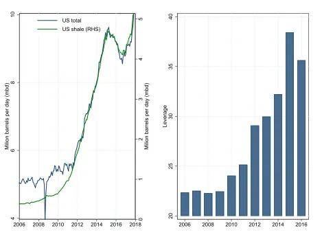
We are first to analyze hedging practices by oil producers in the decade following the adoption of shale technologies. In this period the surge in production was phenomenal: U.S. crude oil production almost doubled from around 5 million barrels per day (mbd) in 2006 up to about 10.5 mbd in early 2018 (see Figure 1). Technological progress in this decade may have translated also into changes in hedging strategies of oil companies, which have become more akin to an Hotelling producer. For example, as shown byBjornland et al.
(2017) firms using shale oil technology have indeed become more flexible in allocating output intertemporally; by altering their supply response to forward prices at different horizons shale may have changed also their use of derivatives contracts.
0
1
2
3
4
5
Milion
barrels
per
day
(mbd)
4
6
8
10
Milion
barrels
per
day
(mbd)
2006 2008 2010 2012 2014 2016 2018 US total
US shale (RHS)
20
25
30
35
40
Leverage
[image:4.612.82.551.68.413.2]2006 2008 2010 2012 2014 2016
Figure 1
US oil production and leverage
The left plot displays the total US crude oil production and shale oil production measured in terms of million barrels per day (mbd); both series are from EIA. Shale-oil production includes hydraulically fractured production originated from EIA plays: Monterey, Austin Chalk, Granite Wash, Woodford, Marcellus Haynesville Niobrara-Codell, Wolfcamp, Bonespring, Spraberry, Bakken, Eagle Ford, and Yeso-Glorieta. The right plot displays median leverage defined as Total Debt/Assets for selected US E&P companies. Data are from Bloomberg, details on the firms included in the sample are available in Section 3.
low interest rates with fair stable oil prices (Azar, 2017). However, the buildup in leverage was not inconsequential for producers. According toGilje et al.(2017) it materially affected firms output and investment decisions, and could have ultimately made the oil market more exposed to financial shocks (Dale, 2015).
constraints. In the original literature pioneered by Froot et al. (1993) firms engage in hedg-ing because financial constraints make them risk averse. However, this theoretical prediction has been challenged by modern theories of dynamic risk management, claiming that lim-ited or incomplete hedging characterize optimal risk management strategies for financially constrained firms (see Holmström and Tirole, 2000, Mello and Parsons,2000).
More recently Rampini and Viswanathan (2010) and Rampini and Viswanathan (2013) model the dynamic interplay between standard financing and risk management with collat-eral constraints. We focus on oil producers as in this context the functioning of the collatcollat-eral channel is likely to be even more central in explaining risk management practices. First, rev-enues for an oil producer are almost entirely related to the price of oil and gas. Second, the collateral pledged by oil producers takes the form of oil reserves, valued at market prices (see Office of the Comptroller of the Currency, 2018). Our empirical investigation relies on a firm-level dataset of over 100 E&P U.S. oil producers, between 2006 and 2016. We hand-collected data on the notional amount of each hedging contract as well as on the different type of financial contracts, used by each firm to hedge the company annual production. This detailed information provides precious information on risk management both at the extensive margin and at the intensive margin.
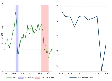
In the aggregate, hedging by US E&P sector recorded a sizable reduction following the two oil price collapses in 2008 and 2014-15. During these two episodes the net worth of oil producers represented in the right plot of Figure 2 was severely impacted. The net income/assets ratio was impaired especially after the 2014-15 slump, where years of accumu-lating leverage combined with a more protracted price downturn made the fragile financial conditions of shale oil producer even more dramatic, and called for a more pronounced at-tention to their financial sustainability by lenders. We use the wide oil price fluctuations as a source of substantial variation in producers risk management strategies, through their effect on firms’ net worth (see the left plot in Figure 2 for the dynamics of the WTI spot price in the last decade).1
Given the substantial oscillations in net worth displayed in our sample, the panel structure of the data allows to exploit both cross-sectional and also siz-able within-firm variation to assess the intensity of the relation between hedging and net worth. We find strong support for a positive causal link between a firm’s net worth and its hedging ratio using both standard and instrumental variable estimation. The results hold both in the cross-section, selecting different sub-samples, as well an in the time series
dimen-1We refer toHamilton(2009),Kilian and Hicks(2012),Kilian(2014),Ellwanger et al.(2017), andPrest
0
50
100
150
O
il
price
US
$
2006 2008 2010 2012 2014 2016 WTI 2008 slump 2014-15 slump
-.3
-.2
-.1
0
.1
[image:6.612.83.551.67.406.2]2006 2008 2010 2012 2014 2016 Net Income/Asset
Figure 2
WTI price and net worth
The left plot displays the West Texas Intermediate (WTI) spot price with shaded area for the two significant oil price collapse in recent years; the series is from Datastream. The right plot displays median net worth defined as Net Income/Assets for selected US E&P companies; details on the firms included in the sample are available in Section3.
sion. Interpreting these two dramatic oil price slumps as quasi-natural experiments, with a difference-in-difference approach we show how the shock to net worth differently affected the risk management practices among oil producers.
of hedging decisions we look into the particular contract chosen to hedge production and we test whether net worth affects not only the hedging intensive margin but also the choice of the specific derivative category.
The rest of this paper is organized as follows. Section 2 reviews some of the theoretical and empirical contributions on firms risk management, Section3 describes the data set and the measures of net worth used to analyze firms’ hedging strategies. Section 4examines the main empirical results and discusses the identification strategy adopted to present evidence of a positive causal link between hedging and net worth. Section6supplements the analysis on hedging and net worth by analyzing how the latter impacts optimal risk management strategies. Finally Section 7 presents our conclusions.
2
Literature review
In the seminal contribution of Froot et al. (1993) firms engage in risk management as a result of costly external financing. By hedging, firms mitigate underinvestment so to ensure sufficient internally generated funds when attractive investment opportunities arise. Despite the appeal of their framework, little empirical evidence has been found for their model (Stulz,
1996).
Still, the same financial constraints motivating risk management may also limit the firms’ ability to hedge. Holmström and Tirole (2000) investigate the determinants of hedging mod-eling jointly liquidity management, risk management and capital structure. The authors suggest that credit constrained firms can preserve internal funds and deliberately choose an incomplete insurance against liquidity shocks to maximize the marginal return on invest-ments in case the shock does actually materialize. Mello and Parsons (2000) characterize optimal hedging strategies for financially constrained firms. In their model the optimal hedge minimizes the variability in the marginal value of the firm’s cash balances, by redistributing them across states and time. Importantly, they emphasize how a poorly conceived hedge can increase the expected costs of financing, tightening the financial constraints and lowering firm value.
forego hedging so to invest its limited resources. Their model is empirically validated in the case of airline companies hedging commodity price risk, see Rampini et al. (2014). Hedging falls among more financially constrained airlines and more so as they approach distress: air-lines prefer to pledge the scarce collateral to finance investments rather than hedging fuel price risk. More recently, Rampini et al. (2017) unveil a similar trade-off between financing and risk management for US financial institutions when hedging interest rate and foreign exchange risk.
A sharp test of the effectiveness of financial risk management for oil producers is provided inGilje and Taillard(2017), who show how hedging is effective in reducing the probability of financial distress and underinvestment risk, thereby affecting also firm value. Following the widening of the spread between US and Canadian oil price benchmarks, Canadian firms more exposed to basis risk are shown to reduce investment, record falling valuations, sell assets, and reduce debt. Focusing on US oil producers, Gilje (2016) studies how collateral based financing may distort investment decisions and trigger risk shifting behavior. He exploits an exogenous variation in leverage, induced by two episodes of marked oil price falls, to show that more restrictive covenants or a shorter duration of debt mitigate the risk-shifting, as proxied by the share of expenses in exploratory drilling over total investment expenditure.
Gilje et al. (2017) use detailed well-level data to unveil a debt related investment dis-tortion which emerges when producers, in the face of falling oil prices and a futures curve in contango, rush to complete wells and exploration in order to increase the value of their collateral, so to improve their credit standing. This acceleration in well completion is more pronounced ahead of regularly scheduled renegotiations with creditors. Similarly, Lehn and Zhu (2016) show that, during 2011-16, more leveraged companies faced with collapsing oil prices and declining investment opportunities, still ramped up production to meet debt re-payments. Such a debt-driven investment distortions may even hinder the downward adjust-ment in oil production as oil prices fall, thus reducing the supply elasticity of the otherwise more price sensitive shale producers.
Bakke et al. (2016), in the context of oil and gas companies, exploits a change in financial accounting standards as a quasi-natural experiment to confirm this negative causal relation.
Adam (2002) models firms’ risk management in an inter-temporal setting to rationalize the firms’ optimal decision in choosing between nonlinear and linear hedging strategies. His predictions are further explored in Adam (2009) who finds that options are prevalent in the gold mining industry, with financial constraints significantly increasing the likelihood of their adoption. Mnasri et al. (017a) and Mnasri et al. (017b) conduct an extensive analysis of the determinants and the value effect of nonlinear strategies for US oil producers. They find support for the risk-shifting model of Fehle and Tsyplakov (2005), documenting a non-monotonic relationship between hedging and proximity to financial distress.
Our data set allows to extend the analysis to the oil market sector in a period including both new conditions in the financial markets (commodity financialization) and new pro-ducers relying on increasing leverage to lead the technological change in the oil production (shale revolution). The last part of this study adds to this literature by conditioning risk management strategies to net worth measures.
3
Data
In this Section we first describe the process of data collection based on hedging disclosure available in firms’annual report. Then, we provide some statistics on the derivative contracts employed to cover oil production and we define our measure of hedging activity. Finally, we present some possible measures of net worth that are used in the following empirical analysis.
3.1
Data sources
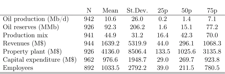
Table 1
Firms’ summary statistics
N Mean St.Dev. 25p 50p 75p Oil production (Mb/d) 942 10.6 26.0 0.2 1.4 7.1 Oil reserves (MMb) 926 92.3 206.2 1.6 15.1 77.2 Production mix 941 44.9 31.2 16.4 42.3 70.0 Revenues (M$) 944 1639.2 5319.9 44.0 296.1 1068.3 Property plant (M$) 926 4136.0 8506.4 133.5 1025.6 3135.8 Capital expenditure (M$) 962 976.6 1948.7 29.0 269.7 923.8 Employees 892 1033.5 2792.2 39.0 211.5 780.5
The table presents summary statistics for US E&P companies. Oil production is crude oil produced measured in thousands of barrels per day; oil reserves is US proven developed and undeveloped reserves of crude oil held by the company at year-end, in millions of barrels;production mix is crude oil production as a percent of the company’s total oil and gas production both measured in terms of barrel of oil equivalent; revenues is oil and gas revenues in US$ millions; property plant is net value of property, land, and other physical capital in US$ millions;capital expenditure is the amount spent on purchases of tangible fixed assets related to E&P activities in US$ millions; employees are firm total employees.
EDGAR, or with less than five years of reports2
. Third, we further filter out smaller report-ing company that are not required to disclose information as their market risk is considered as negligible. This leaves us with 167 unique firms. Finally, we exclude those where risk management practices cannot be reclassified in terms of quantitative data as they are es-sentially not reported in tabular form in item “7A. Quantitative and Qualitative Disclosures about Market Risk”. At the end of this filtering procedure we obtain an unbalanced sample of 102 unique firms observed over an 11 years time period. Some descriptive statistics on oil production, reserves and firm characteristics are shown in Table 1.
The firms in our final dataset account for approximately 30% of overall US oil produc-tion and are especially representative of shale producers.3
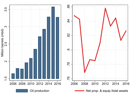
This can be better grasped by comparing production obtained from our firm-level dataset with the one obtained from the US EIA statistics for shale regions. The evolution of production in the right plot of Figure3
closely tracks the one of shale oil production presented in Figure 1, corroborating our choice of the sample to study firms which adopted shale technology. In the peak year of 2015,
2This last choice is primarily motivated to ensure a minimum coverage of hedging practices over the
period of analysis and make our dataset suitable to study within-firm evolution in risk management.
3Major oil companies are not included in our sample, as they are generally classified in the 2911 SIC
1.
5
2
2.
5
3
3.
5
Milion
barrels
(mbd)
2006 2008 2010 2012 2014 2016 Oil production
.76
.78
.8
.82
.84
.86
[image:11.612.89.553.74.400.2]2006 2008 2010 2012 2014 2016 Net prop. & equip./total assets
Figure 3
Oil production and relevance of oil related assets
The left plot displays the total oil production in mbd of E&P firms included in the sample. The right plot shows the median ratio between net property and equipment over total assets; net prop-erty and equipment include oil and gas properties net of accumulated depreciation, depletion and amortization
production reached 3.5 mbd when measured from our firm-level data, approximately 4.8 in the EIA statistics on shale production.
between dynamic risk management and collateral availability, first described by Rampini et al. (2014). In their empirical application, airline companies need to hedge fuel oil costs, which account on average between 20-30% of total operating costs, and firms pledge their assets (aircrafts) to borrow. In our case, oil producers need to hedge their output, and pledge oil reserves, both of which depend on the oil price.
3.2
Net worth measures
As the primary focus of this study is to test the impact of collateral constraints on hedging activity, we augment the data set to include information about firms’ net worth. In the spirit of Rampini et al. (2014) and Rampini et al. (2017) we use several balance sheet and market-based variables to construct a set of net worth measures. To this end, we combine firms’ hedging data with a comprehensive list of financial and accounting variables retrieved from Bloomberg. We consider the following measures of net worth: net income/assets, the market value of equity (market capitalization), the ratio between the book value of equity and total assets, the book value of assets (size), and two market based measures implied by the Bloomberg Issuer Default Risk model, namely the 5 Year CDS and the 1 year probability of default.4
Descriptive statistics on net worth measures and firm leverage are reported in Table 2. Some net worth measures exhibit larger skewness and heterogeneity as concerns the frequency distribution, more so when considering net income/assets and the two market based indicators retrieved from Bloomberg. For these three measures the sample mean is quite far from the corresponding median and the distribution is quite dispersed. To a large extent this finding results from the two oil price slumps within our sample, which especially impacted on the market measures of net worth. In particular, the negative average value displayed for net income/asset reflects the severe net worth impairment experienced by some E&P companies during the two recent oil slumps reported also in the right plot of Figure2.
3.3
Derivative contracts
A benefit of examining the oil and gas industry is that disclosure of firms’ derivative portfo-lios is remarkable. In particular, most firms provide information on each derivative contract, detailing the notional amount, the contract type, and maturity. Unfortunately this informa-tion is not presented in a standardized fashion, and data needs to be first hand collected and
4In some robustness tests we also try additional net worth measures including: cash dividends/assets,
Table 2
Net worth summary statistics and leverage
N Mean St.Dev. 25p 50p 75p Net Income/Assets 945 -0.08 0.32 -0.09 0.01 0.06 Market cap. 881 6.60 2.14 5.22 6.72 8.15 Size 968 6.78 2.27 5.33 7.21 8.30 Equity/Assets 968 0.45 0.41 0.37 0.48 0.64 Bloomberg 5YR CDS 741 2.65 3.31 0.91 1.64 2.91 Bloomberg 1YR PD 760 1.20 3.14 0.01 0.11 0.81 Leverage 961 0.32 0.34 0.12 0.27 0.42
The table presents summary statistics for various new worth measures: net income/assets is net income divided by assets, market capitalization is log(number of shares*end of year price), size is log(assets), equity/assets is the book value of common equity divided by assets, Bloomberg 5YR CDS is 5 Year credit default swap spread for the company implied by the Bloomberg Issuer Default Risk model, Bloomberg 1YR PD is the probability of default of the issuer over the next 1 year calculated by the Bloomberg Issuer Default Risk model. Leverage is total debt divided by assets.
then reformatted. Starting from companies’ 10-K report, we collect the information about the specific contracts used to hedge oil annual production.5
We then classify hedging instruments reported by companies in 8 distinct categories: fu-tures/forward, swaps, collars, 3-way collars, swaption, call options, put options, and other derivatives including residual contracts. Table 3 displays the distribution frequency of the main class of financial instruments used to cover their 12-month ahead oil production. First of all, the table shows that about one third of the sample firms are not engaged in risk man-agement activities, with a remarkable peak around the 2008 oil slump. Moreover, hedging activity tends to be clustered into a limited number of derivative instruments, namely swaps, collars and three way collars. Finally, the table also shows an apparent variability over time in terms of the hedging strategy. This indicates that firms’ dynamic risk management entails decisions not only with respect to the notional amount to be hedged, but also in terms of optimal derivative contract.6
The second and third columns of Table 3include hedging instruments that are classified
5Being our focus on US oil producers, we only consider derivatives where the WTI is the price benchmark
of the contract. These derivatives represent, for the firms in our sample, the most comprehensive category of contracts adopted to hedge oil production if not the totality itself.
6Firms could in principle enter into derivative transactions to achieve a trading profit: however, from the
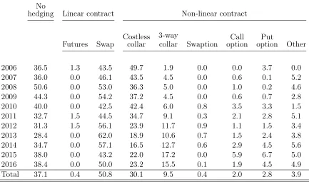
Table 3
Hedging choice and derivative contracts
No
hedging Linear contract Non-linear contract
Futures Swap Costlesscollar
3-way
collar Swaption optionCall optionPut Other
2006 36.5 1.3 43.5 49.7 1.9 0.0 0.0 3.7 0.0 2007 36.0 0.0 46.1 43.5 4.5 0.0 0.6 0.1 5.2 2008 50.6 0.0 53.0 36.3 5.0 0.0 1.0 0.2 4.6 2009 44.3 0.0 54.2 37.2 4.5 0.0 0.6 0.7 2.8 2010 40.0 0.0 42.5 42.4 6.0 0.8 3.5 3.3 1.5 2011 32.7 1.5 44.5 34.7 9.1 0.3 2.1 2.8 5.1 2012 31.3 1.5 56.1 23.9 11.7 0.9 1.1 1.5 3.4 2013 28.4 0.0 62.0 18.9 10.6 0.7 1.5 2.4 3.8 2014 34.7 0.0 57.1 16.5 12.7 0.6 2.9 4.5 5.6 2015 38.0 0.0 43.2 22.0 17.2 0.0 5.9 6.7 5.0 2016 38.4 0.0 50.0 23.2 15.5 0.1 1.9 4.5 4.9 Total 37.1 0.4 50.8 30.1 9.5 0.4 2.0 2.8 3.9
The table displays the frequency of non-hedging firms and the frequency of use of different cate-gories of hedging contracts. The table presents average values computed with respect to all firms reporting in a specific year; all values are in percentage. Category “Other” includes residual hedging instruments such as put spreads, enhanced swaps, fixed-price contracts which are not covered in specific categories.
as linear hedging contracts, i.e futures/forward and swaps. While the frequency of use of futures/forward contracts is marginal or nil for most of the years, swaps represent the most common hedging tool, around 50% over the full sample, peaking at 62% in 2013. The class of nonlinear contracts is very heterogenous: it embraces multiple financial instruments with very different payoff structures. Among these, the importance of costless collars has remarkably shrunk over time, ranging from almost 50% at the start of the period to 23% in 2016. Their decline has been almost entirely offset by the increase in the share of 3-way collars. Plain vanilla instruments, such as call and put options, have gained some use in the most recent years but remain marginal (5% on average in the full sample). Finally, residual financial instruments are used to cover almost 4% of the oil production, while the presence of swaptions is almost insignificant.
.3
.4
.5
.6
.7
Hedging
rat
io
[image:15.612.147.466.74.299.2]2006 2008 2010 2012 2014 2016
Figure 4
Sample hedging ratio
The graph displays the dynamics of the sample average hedging ratio which is defined as the ratio between total notional amounts reported over all hedging contracts to cover the 12 month ahead oil production and the oil production effectively achieved by the firm.
hedged. Rather than an indicator simply signaling the use of derivative contracts (Guay and Kothari, 2003), we construct an indicator measuring the intensive margin of firms’ hedging activity as inHaushalter(2000). More precisely, we start from the notional amounts reported over all hedging contracts to cover the 12 month ahead oil production and define an annual ratio for the fraction of production hedged HR12t as follows:
HR12t=
P
iN otionalit Oil productiont
where N otionalit is the amount of hedged oil barrels for derivative contract i at time t, while Oil productiont represents the annual oil production effectively achieved by the firm. Figure displays the dynamics of the sample average hedging ratioHR12t for the E&P firms
included in the sample. The average share of oil production hedged is 45% across firm-year observations, though with some skewness and variability in the whole sample. Average
HR12t recorded two marked reductions following the oil price slumps (2008 and 2014/15),
management; yet it presents some preliminary empirical evidence of an inverse relationship between the intensity of hedging and oil prices.
4
Hedging and net worth
The key assumption in Rampini and Viswanathan (2010) and Rampini and Viswanathan
(2013) is that collateral constraints apply to both external financing and hedging activity. Hence, managers face a trade-off: they can either engage in hedging motivated by risk aversion concerns or they can preserve resources to increase their investments, more so when firms’ net worth is low and marginal productivity of capital is higher. A vivid example of this trade-off, is provided by the dramatic decision by Continental Resource to settle, in the aftermath of the 2014 oil price slump, all of its derivative contracts prior to expiration. In doing so the company remained completely unhedged and exposed to volatility in crude oil prices, but at the same time was able to cash the gains on its existing derivatives and fund its drilling programs.
In this Section we investigate if and how different measures of firms’ net worth are positively related with firms’ hedging activity. Our specification is based on the following baseline equation:
HR12i,t =α+βN Wi,t+ǫi,t (1)
where for each firm i, HR12 represents the hedging ratio (production hedged as a ratio of
total production) for the 12 month ahead and N W is one of the net worth measures defined in Section 3.2; t denotes time measured in years. In general, if the crowding out effect between hedging and collateralized financing is active, we would expect β to be positive and statistically significant. Clearly, a negative relationship will hold for our market-based measures of default risk, such as Bloomberg 5YR CDS and Bloomberg 1YR PD, which are inversely related to the firms’ net worth.
We present in Table 4 the results for the empirical specifications of interest. All models include firm fixed effects to account for the effect of time-invariant unobserved firm character-istics (e.g. managerial risk aversion, risk management skills) on hedging policies.7
The first column of Table4presents fixed effect panel estimates and provides some strong evidence of
7As a robustness check we also estimate a weighted least square specification and a tobit model to take into
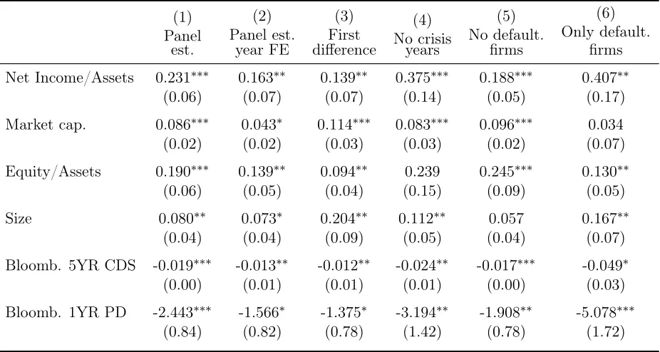
Table 4
Net worth and hedging
(1) Panel est. (2) Panel est. year FE (3) First difference (4) No crisis years (5) No default. firms (6) Only default. firms Net Income/Assets 0.231∗∗∗ 0.163∗∗ 0.139∗∗ 0.375∗∗∗ 0.188∗∗∗ 0.407∗∗
(0.06) (0.07) (0.07) (0.14) (0.05) (0.17) Market cap. 0.086∗∗∗ 0.043∗ 0.114∗∗∗ 0.083∗∗∗ 0.096∗∗∗ 0.034
(0.02) (0.02) (0.03) (0.03) (0.02) (0.07) Equity/Assets 0.190∗∗∗ 0.139∗∗ 0.094∗∗ 0.239 0.245∗∗∗ 0.130∗∗
(0.06) (0.05) (0.04) (0.15) (0.09) (0.05) Size 0.080∗∗ 0.073∗ 0.204∗∗ 0.112∗∗ 0.057 0.167∗∗
(0.04) (0.04) (0.09) (0.05) (0.04) (0.07) Bloomb. 5YR CDS -0.019∗∗∗ -0.013∗∗ -0.012∗∗ -0.024∗∗ -0.017∗∗∗ -0.049∗
(0.00) (0.01) (0.01) (0.01) (0.00) (0.03) Bloomb. 1YR PD -2.443∗∗∗ -1.566∗ -1.375∗ -3.194∗∗ -1.908∗∗ -5.078∗∗∗
(0.84) (0.82) (0.78) (1.42) (0.78) (1.72)
The table presents regression coefficients for the equation relating firms’ hedging ratio and net worth. All models include firm fixed effects. Robust standard error in parentheses. Dependent variable is 12-month ahead hedging ratio. *, **, and *** denote significance at, respectively, the 10%, 5% and 1% level. Net Income/Assets is net income divided by assets, Market Cap. is log(number of shares*end of year price), Size is log(assets), Equity/Assets is the book value of common equity divided by assets,Bloomberg 5YR CDS is 5 Year credit default swap spread for the company implied by the Bloomberg Issuer Default Risk model, Bloomberg 1YR PD is the probability of default of the issuer over the next 1 year calculated by the Bloomberg Issuer Default Risk model. Column 4 displays estimates excluding the years of oil price collapse (2008, 2014, 2015). Defaulted firms include: Berry Petroleum, Emerald Oil, Energy XXI, Escalera Resources, Goodrich Petroleum, Magnum Hunter Resources, Miller Energy Resources, Osage Exploration & Development, Postrock Energy, Sabine Oil & Gas, Sandridge Energy, Stone Energy, Ultra Petroleum.
specification estimated in first differences (column 3). Albeit the statistical and economical significance of our results is somehow weakened, the estimated coefficients still point to a substantial effect across all net-worth measures.
To check whether our results are driven by the years with falling prices, affecting firms’ net worth and forcing managers to reduce hedging and prefer borrowing when collateral is scarce, we also re-estimate the same specification by selecting specific sub-periods. When we exclude the oil price slump years (2008, 2014, 2015), we actually find that the opposite is true, as the standardized effect of net worth on hedging is generally even larger (column 4). In the same spirit, in the last two columns of Table 4we test the model by splitting the sample between firms which never defaulted in our sample (column 5) and those which have defaulted (column 6).8
This is to check if the results reported in columns (2)-(4) are driven by distressed firms included in the sample. Indeed, we would expect defaulted firms to have reduced more intensely their hedging, as collateral constraints become even more binding in this case. The estimates in Columns 5 and 6 seem to rule out also this possibility, though the statistical significance of estimates referred to defaulted firms is not always very strong, which is not surprising in light of the considerably smaller number of observations used.
In general the findings presented in this Section provide, in the context of US oil pro-ducers, a strong empirical validation of the link between net-worth and hedging, emphasized by modern dynamic risk-management theories. This result is remarkably robust both across the range of net-worth measures considered and various model specifications.
5
Tackling endogeneity
In the previous Section we showed that less financially constrained firms engage more in risk management activities. Though this relation seems robust across multiple model speci-fications and definitions of net worth, omitted variable bias and simultaneity may represent a potential concern. In this Section we address this issue. First, we present instrumental variable (IV) estimates using an identification strategy that exploits E&P firms’ main source of net worth, namely oil reserves, as well as a measure of firms’ operational efficiency. Sec-ond, we employ the oil price declines in 2008 and 2014-15 as natural experiments to show how companies remarkably reduced their hedging activity, as they became more financially
8We consider as defaulted the following firms filing for bankruptcy: Berry Petroleum, Emerald Oil, Energy
constrained when hit by these two severe shocks to revenues.
5.1
Instrumental variables estimates
For the IV exercise we focus on net income/assets among the possible measures of net worth. This indicator is a flow variable which successfully captures net worth variations as a consequence of oil price dynamics (see Figure 2). Moreover, to rule out spurious results because of variations in the operating scale of the company, this measure is also standardized by total assets. We consider two possible instruments for net worth. First, we rely on an identification strategy that uses changes in reported oil reserves as a source of idiosyncratic variation in the firms’ net worth.9
Oil reserves account for a substantial fraction of E&P companies’ net worth and represent the principal asset component in their balance sheets, as depicted in Figure 3. Moreover, oil reserves define the common source of collateral in the context of the so called “reserve base lending”, i.e. the standard financing process of E&P firms where the amount of money granted is proportional to the extent of proven oil reserves (Domanski et al., 2015, Azar, 2017). To construct our first instrument, we exploit a unique feature of companies annual reports, which provide detailed information of the factors driving changes in the amount of oil reserves: acquisitions, sales, extensions and new discoveries, production, and revaluation. This allows to discriminate between changes in net-worth due to managerial decisions (e.g. to drill more to expand the reserve base) and hence tightly related to the hedging decision, from those “sufficiently” exogenous to the firms decision. To this end, we only consider the reserve revaluation due to oil price changes and compare this component to the total amount of reserves available to the firm:
Instrument1 = Reserves Revision
Reserves
where Reserves Revision accounts for variations in reserves due to change in commodity prices, and Reserves represent the amount of company’s oil reserves (both variables are measured in physical oil barrels). Our identification strategy is based on the assumption that variation in oil reserves, net of the production component and other recomposition effects driven either by sales or purchases of properties, should affect the intensive margin of hedging through their impact on the firm’s net worth. In fact, oil price dynamics exogenously determines a revaluation of reserves which is unrelated to managerial decisions potentially affecting other firms’ characteristics, such as risk management practices.
Second, as an alternative instrument, we consider a firm-level indicator of efficiency in the exploration activity. We expect more operationally efficient firms to be also the ones with higher net worth. Our identification strategy hinges on the assumption that drilling efficiency, arguably a dimension of productivity relating to the physical and geological characteristics of the oil fields being drilled, while affecting firms’ net worth should not be linked to the financial management decision. To this end, we use the so-called “success rate”, sourced by Bloomberg from financial statements, defined as follows:
Instrument2≡Success rate= Exploration W ells+Develop W ells
Exploration W ells+Develop W ells+Dry Holes
where Exploration Wells is the number of successful new wells drilled to explore for oil and gas reserves, Develop Wells is the number of successful new wells drilled to develop oil and gas production, and Dry Holes is the number of dry holes (unsuccessful attempts) drilled. The success rate represents the percentage of total net wells drilled during the year which found oil or gas deposits in sufficient quantities to merit development. A success rate of 100% would indicate that the company successfully found oil or gas for every new well drilled during the year.10
Our IV estimates (2SLS) are reported in Table 5. The upper panel displays IV estimates using firm fixed effects, while the lower panel shows estimates using first differences; the latter should represent the most appropriate setting to deal with endogeneity being theoretically free of autocorrelation issues. For ease of comparison Table5also reports, in the first column, the estimates obtained earlier when net worth was proxied by net income/assets in Table
4. All specifications are augmented by controlling for a measure of implied volatility of oil prices from the options markets (we use the annual average of the Crude Oil Volatility Index from the Chicago Board of Exchange). Unsurprisingly, crude oil volatility is inversely related to net worth, given the relevance of oil reserves in determining firms’ assets. However, being firm-invariant this measure cannot account for the heterogeneity in net worth. Nevertheless, we include volatility in the list of instruments to test the validity of our identification strategy conditional to oil price changes.
The evidence in Table 5 confirms the theoretical prediction of a positive causal relation linking net worth to hedging. All the IV estimates are qualitatively comparable with those previously reported in Table 4. However, the magnitude of the effect estimated by IV is generally larger than in the one obtained in the panel and first difference estimates. This
10InRampini et al.(2014) the authors instrument net worth with changes in productivity as proxied by
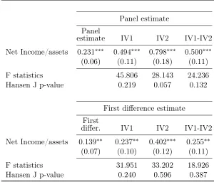
Table 5
IV regression - instrumenting net worth with reserves and success rate
Panel estimate Panel
estimate IV1 IV2 IV1-IV2 Net Income/assets 0.231∗∗∗ 0.494∗∗∗ 0.798∗∗∗ 0.500∗∗∗
(0.06) (0.11) (0.18) (0.11) F statistics 45.806 28.143 24.236 Hansen J p-value 0.219 0.057 0.132
First difference estimate First
differ. IV1 IV2 IV1-IV2 Net Income/assets 0.139∗∗ 0.237∗∗ 0.402∗∗∗ 0.255∗∗
(0.07) (0.10) (0.12) (0.11) F statistics 31.951 33.202 18.926 Hansen J p-value 0.240 0.596 0.387
IV regression with instrumented net worth measure. In Column IV1 the instrument is
Reserve Revision/Reserves , in Column IV2 the instrument is the one year variation in
Suc-cess Rate, while in Column IV1-IV2 both instruments are jointly included in the specification. All
first stage IV regressions also include the annual average of the CBOE Crude Oil Volatility Index (CBOE oil vix). *, **, and *** denote significance at, respectively, the 10%, 5% and 1% level. For IV1 data range is 2010 - 2016 as data on reserves are not widely available before 2010.
result points to possible measurement error attenuation in the panel and first difference es-timates.11
The F-statistics from the reduced form equations points to an adequate relevance of the proposed instruments, while the Hansen J-statistics for the test of overidentifying restrictions never reject the null hypothesis. These tests seem to validate our identification assumptions based on variations to operational efficiency and the value of oil reserves, as two factors affecting risk management practices through their impact on firms’ net worth.
11At least for IV1 where net worth is instrumented via variation in reserves, we stress that a full comparison
5.2
The role of leverage and credit constraints
In the following we shed further light on the relationship between net worth and risk man-agement. To this end, we exploit the two oil price collapses in our sample, i.e. the 2008 and 2014-15 oil price slumps, as quasi-natural experiments. These oil price declines were an exogenous and dramatic shock to oil companies’ net worth which markedly impaired their borrowing capacity. If higher net worth is indeed a key factor driving the interplay between hedging and collateralized external financing, we would expect a decrease in hedging for firms more deeply affected by the commodity shocks. As pointed out byMello and Parsons(2000), every hedging strategy comes packaged with a borrowing strategy. Suggestive evidence for a tight link between between credit and hedging decisions comes from the 2015 10-K filing from Whiting. The credit agreement contains restrictive covenants that may limit our ability to, among other things [...] enter into hedging contracts, incur liens and engage in certain other transactions without the prior consent of our lenders.
We resort to a difference-in-differences strategy (DID), where we separately test the effect of the two price declines by symmetrically splitting our data range in 2011.12
This choice allows to take into account two important issues. First of all, firms may have been differently affected by the two oil collapses, so assuming a dynamic treatment threshold is fundamental for dealing with the time-varying classification of firms (treatment vs control) in the two events and with sample attrition because of bankruptcies. Second, starting from 2010-2011 E&P companies have been facing not only a technological development with shale oil boom, but also a profound transformation of their financial structure as reported in Figure 1. Therefore, by splitting the sample in two periods allows to appreciate the impact of the buildup in debt observed during the shale revolution.
We proceed by assuming a within-event matching, and we construct treatment and control groups on the basis of the companies net worth in the year prior to the crisis. For example, in the DID regression for the 2008 oil slump, a firm is considered as treated when its net worth measured by net income/assets is below the median value of the sample net worth in 2007. A similar strategy is adopted for the 2014-15 case, using the median net worth in 2013.13
The effect of a commodity shock on the hedging ratio of firms is evaluated through a DID setting according to the following regression form:
12The main results discussed in this Section are qualitatively similar with different choices of the splitting
year (e.g. 2010 or 2012) as well as if we exclude observations during the oil slumps years (2008, 2014, 2015). The full set of estimates is available upon request.
13In both episodes we also tried different thresholds for net worth, e.g. percentiles ranging in the interval
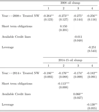
Table 6
Difference in difference estimates
2008 oil slump
1 2 3 4
Year>=2008×Treated NW -0.264∗∗ -0.273∗∗ -0.275∗ -0.256∗∗
(0.123) (0.127) (0.144) (0.116)
Short term obligations 0.150
(0.201)
Available Credit lines -0.011
(0.048)
Leverage -0.251
(0.543)
2014-15 oil slump
1 2 3 4
Year>=2014×Treated NW -0.186∗∗ -0.176∗∗ -0.174∗ -0.182∗∗
(0.093) (0.088) (0.099) (0.091)
Short term obligations -0.113∗∗∗
(0.008)
Available Credit lines 0.066∗∗
(0.027)
Leverage -0.130∗∗
(0.055)
Difference-in-differences estimates with firm fixed-effects. Robust standard error in parentheses. Dependent variable is 12-month ahead hedging ratio. A firm is considered as treated when its net worth measured by net income/assets is below the median value in the year prior to the 2008 or 2014-15 oil price shocks, respectively. Short term obligations represent all debt and payments due within one year,available credit lines represent the unencumbered fraction of credit lines granted to the firm,leverageis measured as total debt/assets *, **, and *** denote significance at, respectively, the 10%, 5% and 1% level.
HRi,t=α+β1P ost+β2T reatment+β3T reatment×P ost+ǫi,t (2)
measures the difference between pre-shock and post-shock hedging behavior for treated firms relative to firms whose net worth is less harshly affected by the decline in oil prices. Table
6 displays the DID estimates for the two episodes, with the 2008 results in the top panel and those for 2014-15 in the bottom panel, respectively. Bearing in mind that oil-related assets account for the lion’s share in E&P companies net worth we would expect, in line with theoretical predictions, the interaction coefficients (β3) to exhibit a negative and statistically
significant sign. This is indeed what emerges from Table6, confirming the causal link between net worth and hedging. In both episodes, the magnitude of the effect is also economically relevant and comparable to the one reported in Table4.
Table 7
Placebo tests
Placebo test
1 2 3 4
Year>=2010×Treated placebo -0.001 0.003 -0.001 0.063
(0.084) (0.086) (0.085) (0.099)
Leverage 0.354
(0.267)
Short term obligations -0.071
(0.378)
Available Credit lines 0.050
(0.048)
Difference-in-differences estimates with firm fixed-effects. Robust standard error in parentheses. Dependent variable is 12-month ahead hedging ratio. A firm is considered as treated when its net worth measured by net income/assets is below the median value in 2010. Estimation sample is 2009-2013 for the placebo test. *, **, and *** denote significance at, respectively, the 10%, 5% and 1% level.
up also directly in the leverage variables, while earlier the same effect was not apparent.14
To check the validity of our quasi-natural experiment and validate the causal interpreta-tion of results, we end this Secinterpreta-tion by presenting the results of a placebo test. We restrict the sample to the period 2009-2013 and create a placebo event in 2011 to examine if treat-ment and control firms engage differently in risk managetreat-ment also in time periods where no relevant oil price decline occurs. In this case a firm is considered as treated if its net worth measured by net income/assets is below the median value of the sample net worth in 2010. Results for the placebo test are displayed in Table7. The interaction terms are always not statistically significant and also considerably smaller in terms of magnitude compared to the estimates reported in Table 6, pointing to no relevant differences in risk management activities among treated and control companies conditional to their level of net worth.
14Smith and Stulz(1985) suggest that direct and indirect cost of bankruptcy should be a key determinant
6
Optimal hedging strategy and net worth
The previous Sections provided extensive evidence of net worth as a major determinant of firms’ hedging decision, an effect amplified when the value of firms’ collateral is impaired by severe oil shocks. In this Section we examine more in detail how optimal hedging strategy and the extensive margin of risk management activities interact with firms’ net worth, an aspect often neglected in previous studies on commodity producers.15
Nevertheless, as shown in Table3, preferences of firms between linear and nonlinear strategies as well as their choice in terms of specific derivative contracts have evolved over time.
Financial derivatives adopted by E&P firms to hedge oil production differ both with respect to their final payoff structure and in costs, as well as in how they can affect the firms’ collateral needs. To the best of our knowledge the only papers specifically devoted to the analysis of the optimal hedging mix in the oil industry are the one byMnasri et al.(017a) and Croci et al. (2017). We depart from their approach from several perspective. First, as previously discussed, we fit our analysis in the framework of dynamic risk management theories, where collateral constraints impinge on the firm ability to engage in derivatives trading. Hence, we explicitly condition the choice of hedging (the extensive margin) to net worth, as well as to financial constraints. Second, we are the first to examine oil producers hedging strategies in the aftermath of the shale technology. As discussed in Section 1 this transformation not only altered the production from the technological point of view, but also the firms’ financial structure.
We focus on the extent of linear hedging measured as oil production covered via linear contracts over total oil production hedged. In this way, we construct an indicator of hedging strategies which is normalized to one, so the natural complement to linear hedging includes all the remaining oil production hedged via collars, three-way-collars, put options, call op-tions, swaption and other residual contracts. We investigate the extent of linear hedging instead of considering specific nonlinear strategies in the spirit ofAdam (2009). Linear con-tracts represent a definitely more homogeneous category and their analysis does not require to distinguish among nonlinear contracts with very different payoffs and underpinning strate-gies.16
Moreover, the heterogeneity among nonlinear contracts does not always support a
15Several authors presented a theoretical framework for the choice of the hedging strategy seeSmith and
Stulz (1985), Adler and Detemple (1988), Froot et al. (1993), Brown and Toft (2002), and Adam (2002) among many others.
16For example, a costly short put with no upside cap is typically adopted for insurance purposes, while
Table 8
Hedging choice and derivative strategy
Income/
Asset MarketCap.
Equity/
Asset Size CDS Default1 year Outcome equation
Net worth 0.048 -0.038∗∗∗ 0.004 -0.037∗∗ -0.005 0.016∗∗
(0.072) (0.012) (0.170) (0.015) (0.007) (0.006) Oil price 0.318∗∗∗ 0.350∗∗∗ 0.288∗∗∗ 0.284∗∗∗ 0.381∗∗∗ 0.399∗∗∗
(0.101) (0.097) (0.096) (0.096) (0.109) (0.104) Production uncert. 0.128∗ 0.088 0.128∗ 0.080 0.299∗∗∗ 0.284∗∗∗
(0.071) (0.073) (0.074) (0.073) (0.087) (0.086) Investments -0.132∗∗∗ -0.120∗∗∗ -0.134∗∗∗ -0.142∗∗∗ -0.223∗∗ -0.216∗∗
(0.045) (0.042) (0.046) (0.048) (0.094) (0.087) Profit diversif. -0.308∗∗∗ -0.379∗∗∗ -0.283∗∗∗ -0.338∗∗∗ -0.396∗∗∗ -0.366∗∗∗
(0.097) (0.098) (0.098) (0.099) (0.109) (0.103)
Leverage 0.212 0.222 0.249 0.262∗ 0.426∗∗ 0.366∗∗
(0.171) (0.145) (0.183) (0.136) (0.187) (0.181)
Leverage2 0.075 -0.006 0.017 -0.008 -0.039 -0.071
(0.103) (0.069) (0.070) (0.067) (0.114) (0.118) Stock options -0.034∗∗ -0.032∗∗ -0.035∗∗ -0.028∗ -0.016 -0.011
(0.015) (0.015) (0.015) (0.015) (0.019) (0.020) Dividends 0.015∗ 0.032∗∗∗ 0.014 0.027∗∗∗ 0.025∗∗∗ 0.024∗∗∗
(0.009) (0.009) (0.008) (0.010) (0.009) (0.009) Selection equation
Net worth 0.680∗∗∗ 0.202∗∗ 1.972∗∗∗ 0.298∗∗ -0.031 -0.151∗∗∗
(0.257) (0.102) (0.580) (0.133) (0.034) (0.044)
Oil price -0.076 0.003 0.136 0.038 0.060 -0.031
(0.419) (0.444) (0.422) (0.428) (0.457) (0.448) Oil production 8.258∗∗ 7.087∗ 7.503∗∗ 5.631 8.140∗∗ 7.512∗
(3.792) (3.787) (3.767) (3.442) (3.841) (3.883) Investments -0.450 -0.527 -0.778∗ -0.514 -1.134∗∗∗ -1.263∗∗∗
(0.372) (0.385) (0.435) (0.339) (0.426) (0.425) Profit diversif. 0.921∗ 1.283∗∗ 0.837∗ 1.023∗∗ 0.605 0.469
(0.475) (0.583) (0.506) (0.493) (0.535) (0.477)
Leverage 3.347∗∗∗ 2.947∗∗ 3.793∗∗∗ 2.844∗∗ 2.015 2.936∗∗
(1.102) (1.223) (1.228) (1.133) (1.274) (1.147) Leverage2 -2.717∗∗∗ -3.266∗∗∗ -1.814∗∗ -2.557∗∗∗ -1.764∗∗ -2.120∗∗
(0.912) (1.007) (0.888) (0.932) (0.862) (0.847)
Stock options 0.204∗ 0.167 0.218∗ 0.212∗ 0.172 0.206∗
(0.123) (0.121) (0.126) (0.124) (0.118) (0.121)
Dividends 0.178∗ 0.091 0.217∗∗ 0.158 0.155 0.160
(0.096) (0.109) (0.093) (0.103) (0.104) (0.103)
Robust standard error in parentheses. In the selection equation, the dependent variable is equal to 1 when the firm is engaged in risk management activities. In the outcome equation the dependent variable measures the extent of linear notional over total amount of notional hedged. The header of each column indicates the measure of net worth that is used in the estimation, see the text for precise definitions. Average oil
is the annual average of the WTI oil prices, Production uncertainty is the coefficient of variation of firm oil production, Oil production is the amount of crude oil produced by the firm in thousands of barrels per day, Investment is defined as firm’s capital expenditure over net property, plant, and equipment, Leverage
clear-cut identification of the main determinants of the optimal hedging strategy, and the available empirical findings are sometimes inconclusive to this purpose, see Adam (2009) or
Croci et al. (2017). This could be even more problematic for some categories of nonlinear derivatives whose use is almost minimal in specific sample years (see Table 3).
We estimate a Heckman model to control for sample selection in the hedging decision.17
In the first stage, the dependent variable is a binary dummy equal to 1 when the company’s 10-K reports derivative contracts in place to hedge oil production. In the second stage, we evaluate the preference for linear hedging by measuring the extent of total notional hedged through linear contracts over the total notional amount of the hedging portfolio; in both stages we include one measure of net worth and we control for several variables which have been identified to play a role in shaping risk management strategies. The estimates are presented in Table 8, with the selection equation in the bottom panel and the outcome equation in the top panel.
Our selection equation results confirm the cross-sectional and panel evidence on the role of net worth presented in Section 4, except when we use the 5 year CDS measure which is still negative but not statistically significant. On the other hand, collateral constraints seem to influence only marginally the decision about the optimal amount of linear contracts. In the outcome equation, a higher net worth is associated with a smaller share of linear hedging, though this result is not uniform and depends on each specific measure. As a possible explanation, linear hedging could be preferred by firms with lower net worth as it does not necessarily require an upfront premium. Conversely, a higher net worth could drive firms towards more complex and expensive nonlinear strategies, which however preserve the upside potential. Alternatively, the risk management function could be less developed and skilled in firms with lower net worth, thus explaining their preference for naive derivative strategies.
The impact of the oil price on the decision of whether to hedge is never significant; on the contrary, and not surprisingly, increasing levels of oil production positively affects the probability to enter a derivative contract. Oil price is also found to be strongly positively correlated with the extent of linear hedging. Linear contracts such as swap and forwards allows firms to hedge their production but they do not represent a profitable strategy when oil prices increase because of a cap to the upside potential with respect to nonlinear strate-gies, a result already documented in Adam (2002) and Adam (2009) for gold mining firms.
17For the sake of brevity the analysis in the previous sections ignored the selection bias for hedging as our
Production risk, defined as firm-specific coefficient of variation of oil production, is positively associated with the extent of linear contracts. Brown and Toft(2002) andGay et al.(2002) show that when firms’ risk spectrum widens to include additional non-hedgeable risk such as production uncertainty, then risk managers should increase their exposure to nonlinear contracts, a result which is empirically found also in Mnasri et al. (017a).18
Capital expenditures measuring firms’ investment propensity are negatively correlated with risk management activities and with the use of linear contracts. Froot et al. (1993) show that firms with large investment programs should be active hedgers, with the amount of nonlinear contracts increasing in the nonlinearity of capital expenditures. Our estimates do not confirm the first prediction, and underscore again the relevant trade-off between hedging and investments. On the contrary, we confirm the second prediction, particularly fitting for E&P companies where investment programs are highly nonlinear and strongly dependent on oil prices. We also find that less diversified firms are more likely to engage in financial hedging, consistent with the absence of other forms of diversification via either natural or operational hedging. In addition, our results suggest that a lower industrial diversification is also strongly associated with the use of nonlinear contracts. More diversified firms could be more flexible in halting production with adverse oil market conditions. In turn this translates in their resorting more to nonlinear hedging strategies.
Leverage is found to be a significant determinant of the choice to initiate a derivative strategy19
, with the lower panel of Table 8 showing a clear non linear relationship: more leveraged producers are increasingly likely to hedge, but when closer to default the sign of this relationship changes. This result could be explained via the so-called option to default: firms facing very high distress costs avoid hedging and divert money to new projects instead of preserving value for bondholders, because of the limited liability condition.
A managers’ convex compensation scheme, proxied by the use of stock options, is neg-atively related to the use of linear contracts in line with theoretical predictions outlined in
Smith and Stulz (1985). Finally, cash dividends exhibit a positive effect on the probability of hedging though the estimates in the selection equation are not always statistically signif-icant. On the contrary, the results in the outcome equation generally indicate an increasing
18This finding should be interpreted with some caution as this variable actually resembles more to a sort
of firm fixed-effect rather than a time varying measure of production uncertainty. For the same reason we exclude, after testing for their statistical significance, similar regressors from the empirical specification such as price-quantity correlation or the correlation between oil price and firm cash flows, suggested by Froot et al.(1993),Gay et al.(2002), andBrown and Toft(2002) among others.
19Results are qualitatively similar when we substitute leverage with alternative indicators of firms’
extensive margin achieved through linear contracts for firms with wealthy dividend policies (Adam,2009).
7
Conclusions
References
Adam, T. (2009), “Capital expenditures, financial constraints, and the use of options,” Jour-nal of Financial Economics, 92, 238 – 251.
Adam, T. R. (2002), “Risk management and the credit risk premium,” Journal of Banking & Finance, 26, 243–269.
Adler, M. and Detemple, J. B. (1988), “On the Optimal Hedge of a Nontraded Cash Position,”
Studies in Banking and Finance, 5, 181–197.
Azar, A. (2017), “Reserve Base Lending and the Outlook for Shale Oil and Gas Finance,” Columbia Center on Global Energy Policy working paper.
Bakke, T.-E., Mahmudi, H., Fernando, C. S., and Salas, J. M. (2016), “The causal effect of option pay on corporate risk management,” Journal of Financial Economics, 120, 623 – 643.
Bjornland, H. C., Nordvik, F. M., and Rohrer, M. (2017), “Supply Flexibility in the Shale Patch: Evidence from North Dakota,” .
Brown, G. W. and Toft, K. B. (2002), “How Firms Should Hedge,” The Review of Financial Studies, 15, 1283–1324.
Croci, E., Giudice, A., and Jankensgård, H. (2017), “CEO Age, Risk Incentives, and Hedging Strategy,” Financial Management, 46, 687–716.
Dale, S. (2015), “New Economics of Oil,” Society of Business Economists Annual Conference, London.
Domanski, D., Kearns, J., Lombardi, M., and Shin, H. (2015), “Oil and Debt,” BIS Quarterly Review March 2015, pp. 55–65.
Ellwanger, R., Sawatzky, B., and Zmitrowicz, K. (2017), “Factors Behind the 2014 Oil Price Decline,” pp. 1–13, Bank of Canada Review.
Fehle, F. and Tsyplakov, S. (2005), “Dynamic risk management: Theory and evidence,”
Journal of Financial Economics, 78, 3 – 47.
Gay, G. D., Nam, J., and Turac, M. (2002), “How firms manage risk: the optimal mix of linear and non-linear derivatives,” Journal of Applied Corporate Finance, 14, 82–93.
Gilje, E. P. (2016), “Do Firms Engage in Risk-Shifting? Empirical Evidence,” Review of Financial Studies, 29, 2925–2954.
Gilje, E. P. and Taillard, J. P. (2017), “Does Hedging Affect Firm Value? Evidence from a Natural Experiment,” The Review of Financial Studies, 30, 4083 – 4132.
Gilje, E. P., Loutskina, E., and Murphy, D. (2017), “Drilling and Debt,” Darden Business School Working Paper No. 2939603.
Guay, W. and Kothari, S. (2003), “How much do firms hedge with derivatives?” Journal of Financial Economics, 70, 423 – 461.
Hamilton, J. D. (2009), “Causes and Consequences of the Oil Shock of 2007-08,” Working Paper 15002, National Bureau of Economic Research.
Haushalter, G., Heron, R. A., and Lie, E. (2002), “Price uncertainty and corporate value,”
Journal of Corporate Finance, 8, 271 – 286.
Haushalter, G. D. (2000), “Financing Policy, Basis Risk, and Corporate Hedging: Evidence from Oil and Gas Producers,” The Journal of Finance, 55, 107–152.
Holmström, B. and Tirole, J. (2000), “Liquidity and Risk Management,” Journal of Money, Credit and Banking, 32, 295–319.
Jin, Y. and Jorion, P. (2006), “Firm Value and Hedging: Evidence from U.S. Oil and Gas Producers,” The Journal of Finance, 61, 893–919.
Kilian, L. (2014), “Oil Price Shocks: Causes and Consequences,” CEPR Discussion Papers.
Kilian, L. and Hicks, B. (2012), “Did Unexpectedly Strong Economic Growth Cause the Oil Price Shock of 2003-2008?” Journal of Forecasting, 32, 385–394.
Lehn, K. and Zhu, P. (2016), “Debt, Investment and Production in the U.S. Oil Industry: An Analysis of the 2014 Oil Price Shock,” SSRN working paper.
Mnasri, M., Dionne, G., and Gueyie, J.-P. (2017a), “The use of nonlinear hedging strategies by US oil producers: Motivations and implications,” Energy Economics, 63, 348–364.
Mnasri, M., Dionne, G., and Gueyie, J.-P. (2017b), “Dynamic corporate risk management: Motivations and real implications,” Journal of Banking & Finance.
Office of the Comptroller of the Currency (2018), “Comptroller’s Handbook: Oil and Gas Exploration and Production Lending,” .
Prest, B. C. (2018), “Explanations for the 2014 oil price decline: Supply or demand?” Energy Economics, 74, 63 – 75.
Rampini, A. A. and Viswanathan, S. (2010), “Collateral, Risk Management, and the Distri-bution of Debt Capacity,” The Journal of Finance, 65, 2293–2322.
Rampini, A. A. and Viswanathan, S. (2013), “Collateral and capital structure,” Journal of Financial Economics, 109, 466 – 492.
Rampini, A. A., Sufi, A., and Viswanathan, S. (2014), “Dynamic risk management,” Journal of Financial Economics, 111, 271 – 296.
Rampini, A. A., Viswanathan, S., and Vuillemey, G. (2017), “Risk Management in Financial Institutions,” Duke University working paper.
Smith, C. W. and Stulz, R. M. (1985), “The Determinants of Firms’ Hedging Policies,” The Journal of Financial and Quantitative Analysis, 20, 391–405.
Stulz, R. M. (1996), “Rethinking risk management,” Journal of Applied Corporate Finance, 9, 8–25.