Classification of bird species from video using appearance and motion features

(1)

Classification of bird species from video using appearance

and motion features

ATANBORI, John, DUAN, Wenting, SHAW, Edward, APPIAH, Kofi

<http://orcid.org/0000-0002-9480-0679> and DICKINSON, Patrick

Available from Sheffield Hallam University Research Archive (SHURA) at:

http://shura.shu.ac.uk/22060/

This document is the author deposited version. You are advised to consult the

publisher's version if you wish to cite from it.

Published version

ATANBORI, John, DUAN, Wenting, SHAW, Edward, APPIAH, Kofi and DICKINSON,

Patrick (2018). Classification of bird species from video using appearance and

motion features. Ecological Informatics, 48 (2018), 12-23.

Copyright and re-use policy

See

http://shura.shu.ac.uk/information.html

(2)

Classification of Bird Species from Video Using Appearance and Motion

Features

John Atanboria,∗_{, Wenting Duan}b_{, Edward Shaw}d_{, Kofi Appiah}c_{, Patrick Dickinson}b

a_{University of Nottingham, School of Computer Science, Nottingham, UK} b_{University of Lincoln, School of Computer Science, Lincoln, UK} c_She_ffi_{eld Hallam University, Department of Computing, She}_ffi_{eld, UK} d_{Don Catchment Rivers Trust, St Catherines House, Woodfield Park, Doncaster, UK}

Abstract

The monitoring of bird populations can provide important information on the state of sensitive ecosystems; however, the manual collection of reliable population data is labour-intensive, time-consuming, and potentially error prone. Au-tomated monitoring using computer vision is therefore an attractive proposition, which could facilitate the collection of detailed data on a much larger scale than is currently possible.

A number of existing algorithms are able to classify bird species from individual high quality detailed images often using manual inputs (such as a priori parts labelling). However, deployment in the field necessitates fully automated in-flight classification, which remains an open challenge due to poor image quality, high and rapid variation in pose, and similar appearance of some species. We address this as a fine-grained classification problem, and have collected a video dataset of thirteen bird classes (ten species and another with three colour variants) for training and evaluation. We present our proposed algorithm, which selects effective features from a large pool of appearance and motion features. We compare our method to others which use appearance features only, including image classification using state-of-the-art Deep Convolutional Neural Networks (CNNs). Using our algorithm we achieved an 90% correct classification rate, and we also show that using effectively selected motion and appearance features together can produce results which outperform state-of-the-art single image classifiers. We also show that the most significant motion features improve correct classification rates by 7% compared to using appearance features alone.

Keywords: Appearance Features, Motion Features, Feature Extraction, Feature Selection, Bird Species Classification, Fine-Grained Classification

1. Introduction

Fine-grained object classification is a well know chal-lenge in computer vision, and there has been some previ-ous work on bird species recognition using individual im-ages (Gavves et al., 2015; Berg et al., 2014; Berg and Bel-humeur, 2013; Huang et al., 2013; Branson et al., 2014;

∗

Corresponding author:

Email address:john.atanbori@nottingham.ac.uk(John Atanbori)

(3)

opportu-nities: the flight patterns of birds are known to vary across different species (Bruderer et al., 2010; Duberstein et al., 2012) and are used by human observers to assist recog-nition. Very few existing studies (Cullinan et al., 2015; Matzner et al., 2015) have made use of motion features in this way, and these have only differentiated small num-bers of species. None has previously combined appear-ance and motion features to facilitate improved classifica-tion.

We focus on this challenge, and present our system which can reliably classify thirteen bird classes in flight. In our previous work (Atanbori et al., 2016), we presented separate sets of appearance and motion features, and showed that our appearance features out-performed the state-of-the-art (Marini et al., 2013). We further showed in Atanbori et al. (2015) that motion features can be used for real-time classification. In this paper we present the following new contributions:

1. We combine appearance and motion features to clas-sify bird species in flight.

2. We introduce an extended dataset, which contains video data of thirteen bird classes. This presents a significant challenge, and is representative of real-world monitoring contexts.

3. We compare feature selection methods, with four standard classifiers, Random Forest (RF), Random Tree (RT), Naive Bayes (NB), and Support Vector Machines (SVM), and compare performance. 4. We compare our method with two state-of-the-art

deep learning models (VGG19 and MobileNet), which are used to classify individual images from our dataset.

5. We have demonstrated that the most significant mo-tion features improve correct classificamo-tion rate com-pared to using appearance features only.

The remainder of this paper is structured as follows. In Section 2, we review existing work, including appli-cations to other species. In Section 3, we introduce our dataset and processing architecture, then proceed to Sec-tion 4 which describes our moSec-tion and appearance fea-tures. In Sections 4, 5 and 6 we describe our feature se-lection, classifiers, and experimental setup, and conclude in Sections 7 and 8, by presenting our evaluation and re-sults.

2. Related Work

A common approach taken by many computer vision researchers in monitoring and identification of animals is to exploit the feature selection techniques, e.g. (Matzner et al., 2015; Spampinato et al., 2010; Beyan, 2015). Hence, in this section we review relevant papers from this domain, and conclude with a review of feature selection techniques.

2.1. Studies related to other Species

Colour features are generally undetectable in low-light, and so applications to bat monitoring have looked more closely at motion features. For example, Cullinan et al. (2015); Matzner et al. (2015); Hristov et al. (2010); Betke et al. (2008); Lazarevic et al. (2008) censused large bat populations. Betke et al. (2008) also estimated wing beat frequencies of individuals using pose templates, and ap-plying Fast Fourier Transform (FFT). Previous work by ourselves, Atanbori et al. (2013), also used FFT to deter-mine wing beat frequency, but using a bounding box fitted to the segmented silhouette. Like Betke et al., works by Cullinan et al., Matzner et al., and Lazarevic et al. use thermal imaging. Cullinan et al. defined four classes (bat, gull, tern, swallow), and using flight tracks reported 82% correct classification; however, this does not con-sider fine-grained differentiation.

Lee et al. (2003) used shape contour features to dis-criminate between nine fish species, and achieved a classi-fication rate of between 13% and 80%. Spampinato et al. (2010) also used texture and shape features, achieving a 92% correct rate. Rodrigues et al. (2010) used Scale-Invariant Feature Transform (SIFT) and Principal Com-ponent Analysis (PCA), achieving similar results to Lee et al., and Spampinato et al. (92% across six species).

2.2. Classification of Bird Species

(4)

methods use colour and shape features, without consid-ering their relative position or orientation (Marini et al., 2013; Wah et al., 2011a,b). For example, Marini et al. uses colour features with SVM. Again, these have been used to differentiate between small numbers of species, and struggle to maintain performance as the number in-creases. Marini et al. showed that when using colour fea-tures alone on the Caltech-ucsd birds-200-2011 dataset, accuracy reduces from approximately 85% when select-ing between 2 species to 20% when differentiating be-tween 17 species.

Part-based methods associate features with specific body parts (Wah et al., 2011a; Duan et al., 2012; Berg and Belhumeur, 2013; Huang et al., 2013; Branson et al., 2014; Wah et al., 2011b; Berg et al., 2014). This can help differentiate between species with high visual cor-relation, but almost all require manual inputs, and good-quality images. Berg et al. developed an online appli-cation called Birdsnap; this requires manual annotation of parts prior to segmentation and classification. Krause et al. (2015), and Gavves et al. (2013, 2015) both de-veloped annotation-free parts-based methods. Their re-sults compared favourably: based on CUB-2011, correct classification rates were 62%, 82% and 67% respectively. They used the Grab-Cut segmentation method (Rother et al., 2004), and so still require some manual interven-tion. Another annotation free method was proposed by Zhang et al. (2015), which detects parts using Convo-lutional Neural Network (CNN). Whereas Krause et al. align the co-segmented objects before labelling, Zhang et al. (2015) uses CNN feature to detects parts automati-cally, but did not improve significantly on other methods. Our objective is to develop a deployable system, capa-ble of identifying birds in flight. Existing methods require manual annotation and/or high quality images which ex-ceed the quality available in real-world settings. In ad-dition, we assert that birds far from the camera are less easily classified using appearance features alone. This motivates our approach of combining colour and motion features. Of the other approaches mentioned, we consider that Marini et al. is an appropriate comparator for this problem domain, being fully automated, non-parts based (so more likely to be robust to reduced image quality), and reporting good results. We therefore use this method as an initial benchmark for our work. Deep learning is the cur-rent state-of-the-art in image classification; we have thus

also used two recent CNN models as additional bench-marks.

2.3. CNN Classification Methods

As mentioned in Section 2.2, Krause et al. and Zhang et al. (2015) used CNN methods for single image species classification. CNN has become prevalent in computer vision for image classification since (Krizhevsky et al., 2012) won the ImageNet Challenge in 2012. Deep learn-ing has been used to achieve state-of-the-art accuracy on ImageNet (Deng et al., 2009), and the PASCAL VOC (Ev-eringham et al., 2012) datasets. Important recent archi-tectures include VGG16 and VGG19 (Simonyan and Zis-serman, 2014), which are very deep networks achieving state-of-the-art classification on the 2014 ImageNet chal-lenge. The original VGG19 model comprised 144 million parameters; however, MobileNets (Howard et al., 2017) is another state-of-the-art deep learning model that uses depth-wise separable and point-wise convolutions to re-duce the number of model parameters (to only 4.2 mil-lion). This model trades accuracy against resources, but still achieved classification accuracy comparable to very deep networks with many large numbers of parameters. We have evaluated our work against both state-of-the-art networks (VGG19 and MobileNet) and presented results in section 7.

2.4. Feature Selection and Reduction

We make extensive use of feature selection and reduc-tion in the method we present in this paper, and so include a short review of relevant techniques here. Redundant or irrelevant features may affect classification rates neg-atively (Hall, 1999; Yu and Liu, 2003). Thus, feature re-duction may be important for fine-grained identification. Existing feature selection methods can broadly be divided intofilterandwrappermethods.

(5)

Wrapper methods use machine learning to evaluate the effectiveness of feature subsets (Tang et al., 2014). An ex-ample was proposed by Breiman (2001), and is based on Variable Importance (VI) derived from Classification and Regression Trees (CART), and Random Forests. How-ever, if the data contains groups of correlated features of similar importance, then smaller groups are favoured (Tolos¸i and Lengauer, 2011). Hall (1999) and Hall et al. (2009) proposed some methods to combine the filter and wrapper methods. Hall reported the performance and ac-curacy of this approach to be better than wrappers on some datasets.

3. Dataset and Preprocessing

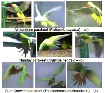
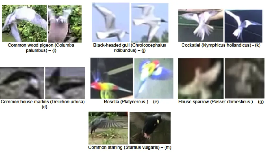
[image:5.612.95.277.459.620.2]

Figures 1, 2 and 3 show samples from our video dataset, recorded using a Casio Exilim ZR100 camera at 240 frames per second. There are thirteen classes in total, made up of ten unique species and another (Melopsitta-cus Undulatus) with three colour variants. The dataset is made up of videos recorded over several days, from three different sites and each class is made up of at least ten individuals. Table 1 shows the number of videos and im-ages per species. The majority (most represented) class is the Black-headed Gull (Chroicocephalus ridibundus), and the minority is the Common wood pigeon (Columba palumbus).

Figure 1:Parakeet samples from our dataset. a)Alexandrine para-keet (Psittacula eupatria),b)Nanday parakeet(Aratinga nenday) andc)

Blue-crowned parakeet (Thectocercus acuticaudatus)

Figure 2:Budgerigar samples from our dataset. f)Budgerigar (yel-low) (Melopsittacus undulatus),h)Budgerigar (wild-type) ( Melopsitta-cus Undulatus) andl)Budgerigar (blue) (Melopsittacus Undulatus)

For each frame in each video, we automatically ex-tracted the target bird silhouette (Fig. 4) using a back-ground Gaussian Mixture Model (GMM) (Zivkovic and van der Heijden (2006)). We used the method proposed by Suzuki et al. (1985) to obtain contours and oriented bounding boxes. A selection of metrics (height, width and hypotenuse, centroid, silhouette and contour points) was automatically determined. We also extracted and con-catenated colour moments, shape moments, greyscale his-togram, Gabor filter and log-polar features (see Section 4). For motion features, we formed a trajectory with the 2D centroid position, described as:

T ={(x1,y1), . . . ,

xj,yj

, . . . ,(xN,yN)} (1)

WhereNis the number of frames inT, represented as a series ofxandycoordinates. We segmented the trajectory (Equation 1) into overlapping sub-trajectoriestkof equal

length, wherek=1. . .N−Q+1 is the total number of sub-trajectories:

(6)

[image:6.612.90.520.122.369.2]

Figure 3:Other samples from our dataset. d)Common house martin (Delichon urbica),e)Eastern Rosella (Platycercus eximius),g)House sparrow (Passer domesticus),i)Common wood pigeon (Columba palumbus),j)Black-headed gull (Chroicocephalus ridibundus),k)Cockatiel (Nymphicus hollandicus), andm)Common starling (Sturnus vulgaris)

filter (Gonzalez and Woods, 2002) with a 1 x 3 kernel to reduce noise. We extracted motion features from the set of smoothed short trajectories (see Equation 2).

[image:6.612.309.539.435.571.2]

Figure 4: Flying birds segmented from our data.

Table 1: Number of videos and images of the thirteen classes

Species # of videos # of images # of images/total(%)

j=Black Headed Gull 147 38,764 24% d=Common House Martin 139 25,517 16% a=Alexandrine Parakeet 79 12,801 8%

l=Budgerigar (blue) 81 12,090 7%

g=House Sparrow 78 10,191 6%

b=Nanday Parakeet 60 10,025 6%

m=Common Starling 71 9,865 6%

k=Cockatiels 59 9,398 6%

c=Blue-crowned Parakeet 60 9,076 6%

f=Budgerigar (yellow) 54 7,667 5%

h=Budgerigar (wild-type) 48 6,283 4%

e=Eastern Rosella 44 5,929 4%

i=Common Wood Pigeon 37 4,301 3%

Total 957 161,907 100%

3.1. Additional Preprocessing for CNN Classifiers

For our benchmark comparisons, we used the

[image:6.612.82.288.474.640.2]

(7)

box around the tracked bird’s silhouette. We rescaled the silhouette to a standard size for training and testing. In our case, we used 32x32 image sections, as the majority of the silhouettes in the database are of around this size.

4. Feature Extraction

In this section, we describe a pool of appearance and motion features extracted to form our method, which we did not use in the benchmark methods.

4.1. Appearance Features

Appearance features are collated from existing related works and comprise colour moments and log-polar val-ues, shape moments, Gabor filters and greyscale his-tograms. We have previously shown in Atanbori et al. (2016) that this feature set is useful for bird classification.

4.1.1. Colour Moment Features

Histogram features have been used widely to charac-terise colour images, by constructing histograms across multiple colour channels (Sergyan, 2008; Huang et al., 2010). Statistical features have also been extracted from such histograms and used to describe colour-based tures of bird species. We compute colour moment fea-tures from each bird silhouette by first transforming the colour image from RGB to HSV space, and then building a histogram to represent the distribution of values across each channel. We compute colour moment features by transforming the image from RGB to HSV and forming a histogram of colour values. We use 30 bins for the Hue channel, and 32 each for Saturation and Value, then nor-malise and calculate statistics for each ( Mean, Standard Deviation, Skewness, Energy and Entropy, see Sergyan (2008); Huang et al. (2010)). Each bin value and statistic is used as a single-valued feature, providing 109 in total.

4.1.2. Image Moment Features

Image moments are used in computer vision to find the area (or total intensity) of the segmented object including information about its centroid and orientation. We used spatial moments (Jacob et al., 2001) and Hu moments (Du et al., 2007), to represent the shape of the silhouette in each frame. We first extract the contours (Suzuki and Abe, 1985) followed by the seven Hu moments and ten spatial moments

4.1.3. Greyscale Histogram Features

Greyscale Histogram Features are constructed by first converting the extracted silhouette into a greyscale image. A 256-bin histogram is then created from the greyscale silhouette (excluding background), to form a representa-tion of the greyscale distriburepresenta-tion of pixels. We then com-pute statistics from the bins: mean, standard deviation, skewness, kurtosis, energy, entropy, and Hu’s 2nd_{and 3}rd moments, providing eight features.

4.1.4. Gabor Wavelet Features

Gabor wavelet features have both multi-resolution and multi-orientation properties, are optimal for measuring lo-cal spatial frequencies and yield distortion tolerance space for pattern recognition tasks. The Gabor wavelet trans-form (Lee, 1996) is the convolution between the function gand imageI(x,y), given by Equation 3.

g=exp −x

0₂ +γ2_y0₂ 2σ2

!

exp i 2πx 0

λ +ψ

!!

(3)

wherex0=xcosθ+ysinθ,y0=−xsinθ+ycosθandθ ,λ,ψ,γandσare orientation, wavelength, phase, aspect ratio and standard deviation respectively.

We extract these, using λ = 1, ψ = 0, γ = 0.02,

σ = 1, and Scale = 31. We use four different values forθ={0,π₄,π₂,3π₄}. The result is four greyscale wavelet images, from which we extract mean, standard deviation, skewness, kurtosis, energy, entropy, yielding 20 features.

4.1.5. Log-Polar Features

Pun and Lee (2003) demonstrated that log-polar images can eliminate transformation effects. An imageIis trans-formed into a log-polar formdst(θ,ρ) using Equation 4.

dst(θ, ρ)←src(x,y)f or

      

ρ=logpx2₊_y2

θ=arctanx_yi f x>0 (4)

(8)

4.2. Motion Features

We extracted motion features using a time window de-scribed by Equation 2 and detailed these features in this section.

4.2.1. Curvature Scale Space (CSS)

Both Beyan and Fisher (2013) and Mai et al. (2010) used Curvature Scale Space (CSS) to distinguish trajec-tories; these are robust to noise (Mai et al., 2010), and calculated using Equation 5.

Ki=

x0_iy00_i −y0_ix00_i

x02

i +y

0₂

i

3₂

(5)

wherex0_i,x00_i,y0_iandy00_i are first and second derivatives ofxiandyirespectively.

We formed 22 CSS features which includes ten statis-tics (mean, standard deviation, skewness, kurtosis, en-tropy, minimum, maximum, local minima, local maxima and zero crossings) from the absolute curvature, the num-ber of curves in the CSS image, the total length of all the curves and ten statistics computed from the CSS maxima (as for the absolute curvature). The CSS feature was con-sidered important for two reasons: Firstly, the datasets consist of birds flying in different directions and orienta-tions. Therefore, similar trajectories may appear as a dif-ferent relative orientation with respect to the optical axis. Secondly, they may appear at different scales due to vary-ing distances from the camera.

4.2.2. Turn Based Features

Trajectory turnings were used to represent the shape of flight, and are calculated by computing the slope of the trajectory between consecutive frames. They have been used, similar to those in Li et al. (2006) and Beyan and

Fisher (2013) and were computed using equation 6:

θk=

                                          

arctan(yk−yk−1 xk−xk−1),

if (xk−xk−1)>0.

arctan(yk−yk−1 xk−xk−1)+π,

if (xk−xk−1)≤0,(yk−yk−1)≥0.

arctan(yk−yk−1 xk−xk−1)−π,

if (xk−xk−1)≤0,(yk−yk−1)<0.

(6)

Where (xk −xk−1)2 −(yk−yk−1)2 , 0. A histogram

(with bin of size 3) was used to calculate the ten statistical features, forming a subset of 30 features.

4.2.3. Wing Beat Frequency Features

The periodicity of wings beats is known to vary among bird species (Lazarevic et al., 2008). In Atanbori et al. (2013) we show that for bat species, a bounding box tted to the silhouette of a tracked individual can be used to measure the periodicity of wing beats. We used the same approach in this work and extracted three metrics (height, width and diagonal length) from a bounding box fitted to the bird silhouette. For each frame, we then computed the frequency components of the signal using a sequence of values computed from a time window of N frames, cen-tred on the current frame. Each frequency component is computed using the Fast Fourier Transform (FFT) 7, for each metric separately:

F(k)= (N−1)

X

t=0

f(t)e−i2πkt/N (7)

(9)

be used to increase resolution. Having generated the fre-quency components, the nine most dominant frequencies for each metric (excluding the DC component) were used to form a set of 27 features for the frame.

4.2.4. Centroid Distance Function (CDF)

The centroid distance function (CDF) represents tra-jectory shape (Beyan and Fisher, 2013) and is invariant to translation and rotation. Since the flying bird’s trajec-tory are subject to rotational deformation, we used CDF features which we computed using Equation 8. We then extracted the ten statistical moments (as with the CSS fea-tures) to form this feature set.

CDFi=

q

(xi−xc)2+(yi−yc)2 (8)

where:

xc=

1 N

N−1

X

j=0

xj, yc=

1 N

N−1

X

j=0

yj (9)

i=0,1, ...N−1, andNis the number of points.

4.2.5. Vicinity

We also included normalised vicinity features which were previously used in Liwicki et al. (2006), and cal-culate ten statistical moments from each (Vicinity curli-ness, slope, aspect and linearity) to form a subset of 40. Vicinity features were selected to represent part of the mo-tion features since they consist of features extracted from each point and takes into consideration their neighbouring points and are very robust to noisy data.

4.2.6. Curvature

Birds flight have directional bearings, which can be measured between frames using curvature. The curva-ture is computed as the cosine of the angle between the line from a point to its predecessor, and the fol-lowing line. Given a trajectorytk and successive points

Pk−1,PkandPk+1, the curvature cos (θk) is given by

Equa-tion 10.

cos (θk)=

c2₋_a2₋_b2

2ab (10)

Where: a is the distance from trajectory

point Pk−1(xk−1,yk−1) to Pk(xk,yk) given by

(xk−1−xk)2+(yk−1−yk)2

0.5

. Similarly, b is given

by (xk−xk+1)2+(yk−yk+1)2

0.5

and c is given by

(xk−1−xk+1)2+(yk−1−yk+1)2

0.5

. k = 2. . .Q−1 and Q = 64 is the length of the short trajectory defined in Section 3

Ten statistical features including mean, maximum, minimum, standard deviation, number of zero crossings, local minima and maxima, skewness, energy and entropy of the curvature were extracted.

5. Feature Selection

Our feature set, described in Section 4, totals 320. We hypothesise that some of these are redundant, and have in-vestigated two selection strategies: correlation-based and classifier-based. We describe each below.

5.1. Correlation-based Feature Selection

The correlation-based method is based on Hall et al. (2009). We calculated a matrix of feature-to-class and feature-to-feature Pearsons correlations, and search the subset space (Hall, 1999) to determine the most effective. Themeritsof each feature subset are then computed using equation 11.

Ms=

krc f¯

p

k+k(k−1) ¯rf f

(11)

WhereMsis the merit of k features, ¯rc fis the mean

cor-relation (f ∈ S) and ¯rf f is the average feature-to-feature

inter-correlation. The feature-to-feature correlation can be expressed as:

¯ rf f =

k−1

X

i=1

k

X

j=i+1

rf f{fi,fj}

!

/k_C

2 (12)

Whererf f{fi,fj} is the pairwise correlation of feature fi with fj, andkC2 is the number of combinations possible from the subsetS. The feature-class correlation is calcu-lated as:

¯ rf c=

k

X

i=1

rf c{fi,ci}

!

/k (13)

(10)

5.2. Classifier-based Feature Selection Method

The classifier-based method uses a Random Forest classifier Breiman (2001) with ”Bagging” (Breiman, 1996), Like Breiman (2001), we use permutation impor-tance to calculate tree splits.

6. Experiments

In this section, we describe our experiments, including setup, methodology and benchmarks. For our evaluation we have performed three separate sets of experiments:

• We have quantified the effectiveness of our complete feature set across our dataset using four well-known classifiers.

• Evaluated the two feature selection methods, and have identified the most effective subsets from our pool of features.

• We have compared the results of our method with that of image classification using two deep learning networks (VGG19 and MobileNet).

• We demonstrated that most significant motion fea-tures contribute to classifier effectiveness.

6.1. Setup and Method

For experiments using our proposed method, we com-puted the full set of appearance and motion features for the frames in each video, for each class of bird. These fea-tures were concatenated to create our full feature set (total of 320 features:169 appearance and 151 motion features). We sampled individual image frames from the dataset for all and split the dataset into 80% for training and 20% for testing, which was used to evaluate the effectiveness of the features using four classifiers: the Naive Bayes (NB), Random Forest (RF), Random Tree (RT) and Sup-port Vector Machine (SVM). The SVM classifier is base on LibSVM proposed by Chang and Lin (2011), which is comparable to the one used in Marini et al. (2013) and implemented using a radial basis function kernel. The gamma and cost parameters were optimised using a grid search. We usedK =int(log2(#f eatures)+1) randomly chosen attributes at each node for the RT classifier, with unlimited depth. Convergence of theout of bag errors

for RF occurred at 20 trees. The NB classifier assumed a Gaussian mixture model over the whole training data distribution, one component per class, and estimated pa-rameters from the training data. All our experiments were performed on a Mac book pro laptop running OS X 10.9.5, with 2.5 GHz Processor and 4GB RAM. We used C++with XCode 5.1.1 and OpenCV 3.0 to implement all our pre-processing and feature extraction algorithms and WEKA 3.7 (Hall et al., 2009) for the classification and feature selection algorithms. The results are reported in Section 7.

To investigate performance after feature selection, the correlation-based merits Ms (see Equation 11) were

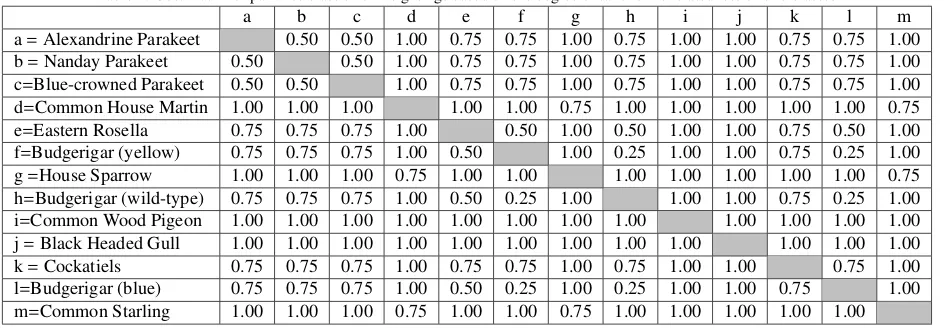
sorted in descending order. Starting with the complete set of 320 features, we iteratively removed the ten least significant until only ten remained, and used the classi-fication rate to plot a learning curve. We used a simi-lar scheme for the classifier-based method and used the curves to identify the optimal parameters and reported the results in Section 7. We applied these techniques to our 169 appearance features only to help to compare our best appearance features to the full feature set and evaluate the contribution of our motion features to classification pformance. We applied a cost matrix of pairwise class er-ror weightings based on the degree of taxonomic relat-edness of the bird classes (see Table 2) for both feature selection and classification. The cost matrix used taxo-nomic relatedness weightings of 0.25, 0.5, 0.75 and 1 for species, family, order and class respectively. We used the approach from Domingos (1999) as it is independent of the actual classifying technique that is used and has a sim-ilar implementation in Weka. The algorithm introduces a bias based on a cost matrixC(i,j) in the training data and predicts the class with the minimum expected misclassifi-cation cost using the values in the cost matrix. Given an example, z and the probabilityP(j|z) of each class j, the Bayes optimal prediction for z is the class i that minimizes the conditional risk in equation 14.

R(i|z)=X

j

P(j|z)C(i,j) (14)

6.2. Benchmarks

(11)

[image:11.612.71.543.140.304.2]

Table 2: Cost matrix of pairwise class error weightings based on the degree of taxonomic relatedness of bird classes.

a b c d e f g h i j k l m

a=Alexandrine Parakeet 0.50 0.50 1.00 0.75 0.75 1.00 0.75 1.00 1.00 0.75 0.75 1.00

b=Nanday Parakeet 0.50 0.50 1.00 0.75 0.75 1.00 0.75 1.00 1.00 0.75 0.75 1.00

c=Blue-crowned Parakeet 0.50 0.50 1.00 0.75 0.75 1.00 0.75 1.00 1.00 0.75 0.75 1.00

d=Common House Martin 1.00 1.00 1.00 1.00 1.00 0.75 1.00 1.00 1.00 1.00 1.00 0.75

e=Eastern Rosella 0.75 0.75 0.75 1.00 0.50 1.00 0.50 1.00 1.00 0.75 0.50 1.00

f=Budgerigar (yellow) 0.75 0.75 0.75 1.00 0.50 1.00 0.25 1.00 1.00 0.75 0.25 1.00

g=House Sparrow 1.00 1.00 1.00 0.75 1.00 1.00 1.00 1.00 1.00 1.00 1.00 0.75

h=Budgerigar (wild-type) 0.75 0.75 0.75 1.00 0.50 0.25 1.00 1.00 1.00 0.75 0.25 1.00

i=Common Wood Pigeon 1.00 1.00 1.00 1.00 1.00 1.00 1.00 1.00 1.00 1.00 1.00 1.00

j=Black Headed Gull 1.00 1.00 1.00 1.00 1.00 1.00 1.00 1.00 1.00 1.00 1.00 1.00

k=Cockatiels 0.75 0.75 0.75 1.00 0.75 0.75 1.00 0.75 1.00 1.00 0.75 1.00

l=Budgerigar (blue) 0.75 0.75 0.75 1.00 0.50 0.25 1.00 0.25 1.00 1.00 0.75 1.00

m=Common Starling 1.00 1.00 1.00 0.75 1.00 1.00 0.75 1.00 1.00 1.00 1.00 1.00

are single image classification using the VGG19 and Mo-bileNet deep networks, which were used to compare our results after feature selection. A Linux server with three GeForce GTX TITAN X GPUs (12 GB memory each) was used to train all the networks. The networks were im-plemented using Python 3.5.3 and Keras 2.0.6 with Ten-sorflow backend. We used all of the images in the dataset with an 80/20 split for training and testing.

We used a transfer learning approach, utilising a ver-sion of the VGG-19 network pre-trained on the Ima-geNet dataset (Krizhevsky et al., 2012). The ImaIma-geNet dataset contains some bird classes, so we reasonably ex-pect higher-level features in the pre-trained network to be applicable to ours. We replaced the input layer with our own (32x32x3) since many of our extracted silhouettes are small. We also replaced the fully connected (FC) layer with our own 13 output classes layer. We also introduced two dropouts, which were used to regularise the network to avoid over-fitting by randomly set a fraction (0.5) of FC layers (fc1 and fc2) units to zero at each update during training. The VGG19 model was trained using a stochas-tic gradient descent (SGD) optimizer, with a learning rate of 0.001 and momentum of 0.9. We used early stopping to interrupt training when the validation loss stops improv-ing, by allowing a patience of 5 epochs. The pre-trained MobileNets model was also used: as with the VGG19 net-work, we removed the input layer (224x224x3) and re-placed it with an input of shape (32x32x3). We rere-placed the FC layer with a new layer and introduced a dropout

(0.5) to regularise the network to avoid over-fitting. Mo-bileNet has the same setup as the VGG-19 network, ex-cept that we reduced the learning rate to 0.0001 and set the two additional hyper-parameters (width and resolution multipliers) to one.

7. Results

Table 3 shows the summary results of the four classi-fiers (NB, RF, RT and SVM) using our full feature set, alongside those obtained using Marini et al.’s features. The results show the overall correct classification rates, which are averaged across the 13 species for each classi-fier.

[image:11.612.308.539.611.673.2]

Table 3 suggests that the Random Forest classifier is su-perior, with the highest correct classification rate based on both our full feature sets and that of Marini et al.. Compar-ing ours with the method used by Marini et al. (2013) also aligns with our previous results in Atanbori et al. (2016).

Table 3: The overall correct classification rates (averaged across 13 classes) usingMarini et. al and our full feature set, without feature selection for the four classifiers.

Marini et. al Our feature Set

Naive Bayes 49% 69%

Random Forest 77% 83%

Random Tree 62% 66%

(12)

We provide a confusion matrix for the RF classifier in Ta-ble 4.

7.1. Feature Selection

As mentioned, we have evaluated two methods of fea-ture selection Hall (1999), and Breiman (2001), using all four classifiers. In this section, we describe how we de-termined the optimal subset and its composition. We used the following procedure to determine the optimal feature subset, for both methods:

• We used the feature selection method to rank the fea-tures.

• We iteratively removed the 10 lowest ranked features from the list.

• For each iteration, we evaluated the performance of each of the four classifiers, using the remaining fea-tures.

• This was repeated until only the 10 highest ranked features remained.

• We plotted a graph of correct classification rates and estimated the maxima for each classifier.

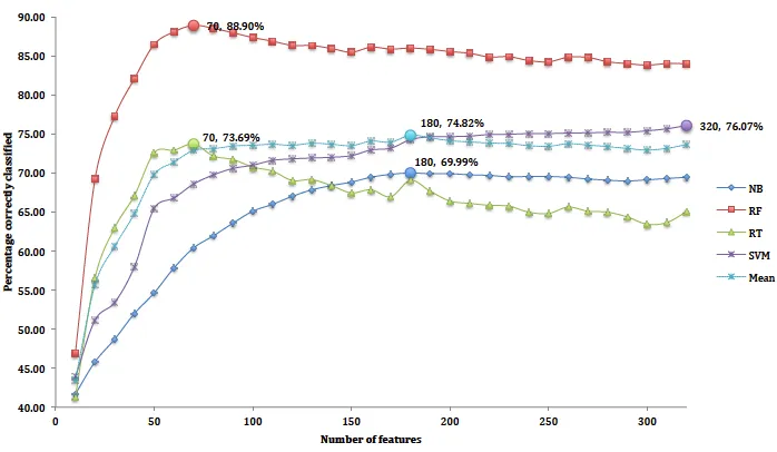
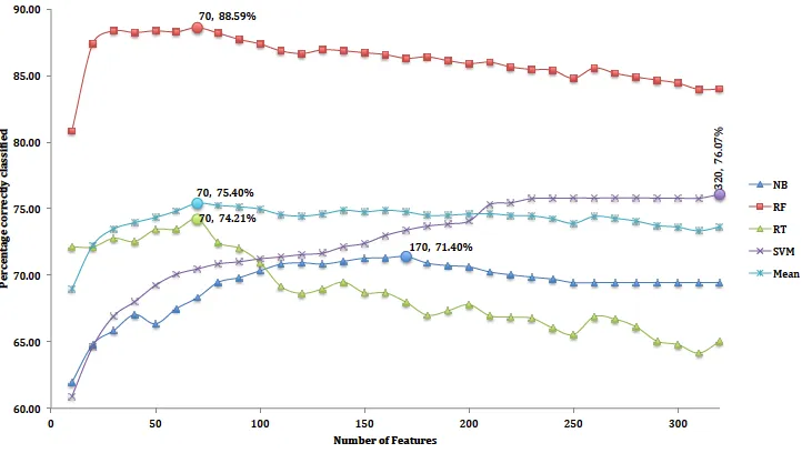
Figures 5 and 6 show the resulting graphs. Each classi-fier is shown as a separate curve. Peaks in the classiclassi-fier- classifier-based method occur at 80 features for RF, 70 for RT and 100 for SVM and NB respectively. Likewise, peaks using the correlation-based method occurred at 80 features for RF classifier, and 70, 90 and 100 for RT, SVM and NB respectively.

We use RF for our analyses as overall it is the best per-forming classifier. Based on the RF, the mode of both fea-ture selection techniques occurred at 70 feafea-tures, which is 89% for the classifier-based method and 90% for the correlation-based method. Table 5 shows feature groups by type, before and after selection, for both methods. The classifier-based method selected 62 appearance features, from four feature groups and the 18 motion features from two groups. The correlation-based method selected 68 ap-pearance features from four groups, and 12 motion fea-tures from one group. Wingbeat frequency was selected by both methods which suggest that they are significant for differentiating species. The highest ranked features

for both classifier-based and correlation-based methods are the width of the FFT peaks (eight width peaks each). These relate directly to the periodicity of wing beats and therefore suggests that flight characteristics may be cru-cial for classifying species.

Birds are usually identified at close distance using their appearances (colour and shape). It is no surprise that most of the features selected were appearance features (62 for the classifier based method and 68 in the case of correlation-based). However, both methods selected only four shape features which strongly suggest the importance of the colour features compared with the shape.

Finally, our proposed feature reduction methods have shown improvement in performance with all classifiers apart from SVM. The results of these are therefore some-what inconclusive, though we note that the improved per-formance with Random Forest is significant in the sense that this is consistently shown as the best classification method (with reduced features, full features, or Marini’s features).

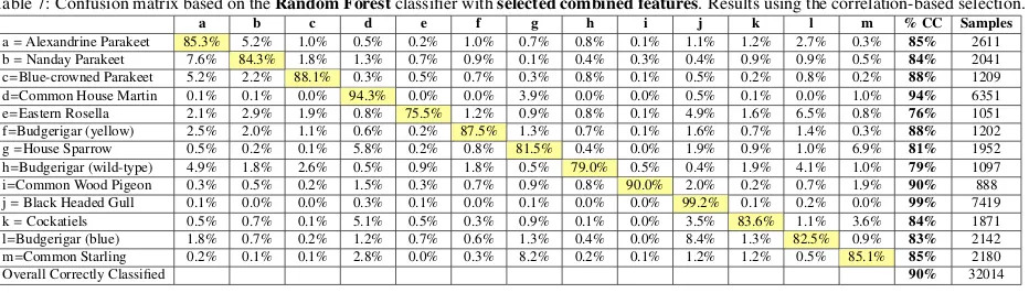
Table 6 shows the results of our full feature set ob-tained using correlation-based feature selection, which summarises the overall correct classification rate for each classifier. We have also provided a confusion matrix for RF (the best performing) in Table 7, to detail misclassifi-cation between species. Overall, the results of our full fea-ture set with feafea-ture selection (90%) outperformed those without (83%), which asserts the efficacy of feature selec-tion.

To help investigate misclassification between species, we considered Order and Family of the birds. We group species into:

1. Four Orders: Psittaciformes(Alexandrine Para-keet, Nanday ParaPara-keet, Blue-crowned ParaPara-keet, Budgerigar (wild-type), Budgerigar (yellow), Budgerigar (blue), Eastern Rosella and Cock-atiel), Charadriiformes(Black-headed Gull),

Columbiformes(Common Wood Pigeon) and

Passeriformes(Common House Martin, Common Starling and House Sparrow).

2. Eight Families: Psittacidae(Alexandrine Parakeet, Nanday Parakeet and Blue-crowned Parakeet),

(13)

(Black-Table 4: The confusion matrix based on theRandom Forestclassifier without feature selection, usingthe combined featureson thethirteen classes dataset (ten bird species and another with three colour forms). %CC is the percentage correctly classified.

a b c d e f g h i j k l m % CC Samples

a=Alexandrine Parakeet 81.2% 6.4% 2.0% 0.5% 0.3% 1.3% 0.6% 0.7% 0.1% 1.8% 1.6% 3.2% 0.4% 81% 2611

b=Nanday Parakeet 9.3% 79.7% 2.4% 1.9% 0.3% 1.4% 0.2% 0.4% 0.3% 0.6% 1.7% 0.9% 0.7% 80% 2041

c=Blue-crowned Parakeet 8.7% 4.2% 82.2% 0.6% 0.4% 0.6% 0.3% 0.7% 0.1% 0.8% 0.2% 0.8% 0.2% 82% 1209

d=Common House Martin 0.1% 0.2% 0.0% 98.7% 0.0% 0.0% 0.3% 0.0% 0.0% 0.4% 0.1% 0.0% 0.2% 99% 6351

e=Eastern Rosella 3.8% 3.9% 2.6% 1.1% 66.3% 1.7% 1.0% 0.6% 0.0% 8.5% 2.8% 7.1% 0.6% 66% 1051

f=Budgerigar (yellow) 5.1% 2.8% 1.5% 1.2% 0.3% 80.9% 1.4% 1.2% 0.1% 2.6% 1.2% 1.2% 0.4% 81% 1202

g=House Sparrow 0.8% 0.1% 0.3% 19.5% 0.4% 0.9% 61.1% 0.5% 0.0% 5.6% 1.1% 1.3% 8.5% 61% 1952

h=Budgerigar (wild-type) 11.2% 4.7% 4.2% 2.9% 1.1% 6.7% 2.9% 47.5% 0.5% 9.6% 4.3% 3.5% 0.9% 47% 1097

i=Common Wood Pigeon 0.9% 1.0% 1.2% 3.3% 0.7% 0.7% 1.8% 0.8% 81.9% 2.4% 0.7% 0.3% 4.4% 82% 888

j=Black Headed Gull 0.1% 0.0% 0.0% 1.7% 0.1% 0.0% 0.1% 0.0% 0.0% 95.0% 1.5% 1.6% 0.0% 95% 7419

k=Cockatiels 1.4% 1.4% 0.1% 9.1% 0.4% 0.5% 1.4% 0.2% 0.1% 5.6% 74.8% 1.7% 3.3% 75% 1871

l=Budgerigar (blue) 2.6% 1.0% 0.3% 2.1% 0.9% 0.5% 1.3% 0.5% 0.0% 16.1% 2.0% 72.5% 0.3% 72% 2142

m=Common Starling 0.9% 0.8% 0.3% 3.9% 0.2% 1.0% 15.3% 0.2% 0.2% 1.2% 2.7% 0.4% 72.8% 73% 2180

[image:13.612.100.514.235.600.2]

Overall Correctly Classified 83% 32014

[image:13.612.130.479.401.604.2]

(14)

[image:14.612.124.485.151.355.2]

Figure 6: Classification rates vs. number of features for correlation-based selection. The maximum for each is marked with a solid circle, and labelled with the number of features.

Table 5: Number of features remaining in each group, before and after applying the classifier-based (CBfs) and correlation-based (CoBfs) Feature Selection, including the top features selected.

Feature Group # before

FS

# after CBfs

# after

CoBfs Top Selected Feature (CBfs) Top Selected Feature (CoBfs)

A

ppearance

Hue color features 37 22 18 σof Hue Mean of Hue

Saturation colour features 35 15 15 Mean of Saturate Mean of Saturate

Value colour features 37 21 31 Entropy of value Entropy of value

Shape 17 4 4 Hu’s First invariant Hu’s First invariant

Gabor 20 0 0 N/A N/A

Grayscale 8 0 0 N/A N/A

LogPolar 15 0 0 N/A N/A

Motion

FFT (Wingbeat) 27 16 12 First Peak of FFT (width) First Peak of FFT (width)

CSS 22 0 0 N/A N/A

CDF 10 0 0 N/A N/A

Turn 62 2 0 Turn (θi=55) N/A

Vicinity 20 0 0 N/A N/A

Curvature 10 0 0 N/A N/A

[image:14.612.70.542.474.648.2]

(15)

headed Gull), Columbidae(Common Wood

Pigeon), Hirundinidae(Common House

Mar-tin), Sturnidae(Common Starling) and Passeri-dae(House Sparrow)

We then aggregate the results from the confusion ma-trices of the thirteen classes to form a four-class order and eight class family confusion matrices (see results in sup-plementary materials). We grouped birds belonging to the same order together to create the order confusion matrices and likewise those belonging to the same family.

The full feature set without feature selection misclassi-fied 9% Columbiformes as Passeriformes whiles this was only 4% with feature selection (see Table 1 in supple-mentary materials). The full feature set also misclassi-fied Psittaciformes as Charadriiformes(6%) and Columb-iformes as PsittacColumb-iformes (6%). These misclassifications reduced to 4% each with feature selection. The worse case misclassifications when considering family without feature selection is Passeridae versus Hirundinidae(19%) and Sturnidae versus Passeridae (15%). Again, with fea-ture selection, these were reduced to 6% and 8% respec-tively.

7.2. Contribution of Motion Features to Classification Rates

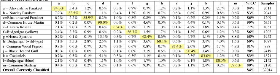
Table 8 shows the results of using appearance versus full-features, with feature selection, which summarises the overall correct classification rate for each classifier. We have provided a confusion matrix for the Random For-est classifier (the bFor-est performing classifier) in Table 11, to detail misclassification between species when we use only appearance features. Results suggest that using both appearance and motion features yields the best classifica-tion rates.

We reconsider the challenge of species recognition us-ing (poor quality) in-the-field data. Our method and those

Table 6: Correct classification rates across all species, with and without correlation-based feature selection (FS) based on the full feature set.

Without Feature Selection With Feature Selection

Naive Bayes 69% 71%

Random Forest 83% 90%

Random Tree 66% 77%

[image:15.612.312.537.153.212.2]

SVM 74% 72%

Table 8: Correct classification rates across all species, with feature se-lection: Appearance versus the full feature set.

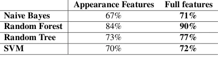
Appearance Features Full features Naive Bayes 67% 71% Random Forest 84% 90% Random Tree 73% 77%

SVM 70% 72%

used for benchmarking are all challenged by similari-ties in appearance between particular species, casting the recognition problem as that of ”fine-grained” classifica-tion. We propose that motion features can act as a weak classifier and assist with differentiation, and there is evi-dence to support this by comparing our combined motion and appearance feature set with that of Marini et al. in Table 3 (our features out-perform those of Marini et al. (2013) with all classifiers).

The contribution of motion features in resolving species may be considered limited with relatively short video clips: however, we note that this is likely to be the case in real in-the-field operation. Furthermore, we re-mark that the retained features in Table 5 include a num-ber of motion features (wingbeat frequencies), which sug-gests that some of these features are significant. Indeed improvements in some species with a similar appearance are evident in Table 7, such as between Parakeet species, and between the Common Starling and House Sparrow. Overall, feature selection with the Random Forest classi-fier introduces a 7% improvement in classification.

(16)

[image:16.612.75.541.136.269.2]

Table 7: Confusion matrix based on theRandom Forestclassifier withselected combined features. Results using the correlation-based selection.

g=House Sparrow 0.5% 0.2% 0.1% 5.8% 0.2% 0.8% 81.5% 0.4% 0.0% 1.9% 0.9% 1.0% 6.9% 81% 1952

k=Cockatiels 0.5% 0.7% 0.1% 5.1% 0.5% 0.3% 0.9% 0.1% 0.0% 3.5% 83.6% 1.1% 3.6% 84% 1871

Overall Correctly Classified 90% 32014

7.3. Results using the VGG19 and MolbileNet Image Classifiers

Tables 9 and 10 show the classification results obtained using the VGG-19 and MobileNet classifiers respectively. The overall correct classification rates for this classifiers were 84% and 80% respectively.

Comparison with the VGG-19 and MobileNet image classifiers are also noteworthy. VGG-19 outperformed MobileNet by 4%, which may be attributed to the fewer parameters of MobileNet since this deep learning model runs on devices with a limited resource (trading-off la-tency against accuracy). Both deep learning methods mis-classified species with a similar shape. However, Mo-bileNet misclassified more of these species than VGG-19. Another interesting observation is that MobileNet net-work misclassified more than 16% of Alexandrine Para-keet as Budgerigar (wild-type). Visualising the higher level filter of this model shows that it relies less on colour than VGG-19, which may explain some differences in per-formance.

Considering the overall classification accuracies us-ing the random forest with feature selection (90% cor-rect classification) outperformed both deep learning ap-proaches. We analyse the results by examining the Order and Family of bird species to investigate this. The worse misclassification for both VGG-19 and MobileNet oc-curred with Psittaciformes versus Passeriformes (4%) and Charadriiformes versus Psittaciformes (5% for MobileNet and 2% for VGG), whiles our approach for these were 3% and 0% respectively. Our method also struggles with Columbiformes versus Passeriformes (4%) but VGG-19 was 3% and MobileNet, 2% for these Orders (see

Ta-bles 7, 9 and 10 in supplementary materials). Again ours misclassified Columbiformes versus Psittaciformes (4%) whiles these were respectively 1% for both VGG-19 and MobileNet. Both Deep Networks misclassified more Families especially Passeridae versus Hirundinidae (22% VGG-19 and 15% MobileNet) and Psittacidae versus Psit-taculidae (12% VGG-19 and 21% MobileNet) whiles ours only misclassified 7% and 4% respectively (see Tables 2, 4 and 5 in supplementary materials). There were very few Families for which the deep learning methods were better than ours.

(17)

[image:17.612.71.549.158.278.2]

Table 9: VGG-19 Confusion Matrix

a b c d e f g h i j k l m %CC Samples

c=Blue-crowned Parakeet 1.57% 1.82% 80.40% 1.24% 3.56% 0.00% 2.65% 1.82% 1.24% 0.74% 1.65% 0.41% 2.89% 80% 1209 d=Common House Martin 0.00% 0.00% 0.02% 96.98% 0.00% 0.00% 1.24% 0.03% 0.00% 0.14% 0.14% 0.00% 1.45% 97% 6351 e=Eastern Rosella 2.09% 2.57% 1.90% 0.10% 70.22% 0.38% 4.57% 3.24% 0.29% 0.29% 2.09% 11.80% 0.48% 70% 1051 f=Budgerigar (yellow) 6.07% 0.42% 1.58% 0.00% 0.08% 82.28% 0.17% 7.90% 0.00% 0.08% 0.00% 1.41% 0.00% 82% 1202

g=House Sparrow 0.05% 0.00% 0.31% 0.87% 0.15% 0.15% 72.59% 0.61% 0.15% 0.10% 0.36% 2.51% 22.13% 73% 1952

j=Black-headed Gull 0.34% 0.05% 0.00% 0.00% 0.31% 0.01% 0.08% 0.03% 0.11% 98.06% 0.23% 0.74% 0.04% 98% 7419

k=Cockatiel 1.87% 0.75% 0.32% 0.27% 2.83% 0.05% 0.91% 3.10% 1.12% 2.67% 74.56% 5.40% 6.15% 75% 1871

[image:17.612.69.549.336.457.2]

Overall Correctly Classified 84%

Table 10: MobileNet Confusion Matrix

a b c d e f g h i j k l m %CC Samples

c=Blue-crowned Parakeet 2.07% 1.41% 82.55% 0.25% 4.14% 0.25% 2.81% 2.73% 0.33% 0.41% 2.32% 0.66% 0.08% 83% 1209 d=Common House Martin 0.00% 0.02% 0.03% 95.10% 0.00% 0.00% 1.97% 0.38% 0.03% 0.03% 1.45% 0.00% 0.99% 95% 6351

g=House Sparrow 0.00% 0.00% 0.20% 2.51% 0.05% 0.46% 75.72% 2.10% 0.31% 0.20% 1.38% 1.69% 15.37% 76% 1952

j=Black-headed Gull 0.04% 0.01% 0.01% 0.04% 0.12% 0.05% 0.61% 0.18% 0.03% 93.95% 1.78% 3.03% 0.15% 94% 7419

k=Cockatiel 0.21% 0.59% 0.00% 0.05% 1.87% 0.21% 3.05% 2.14% 1.07% 2.51% 79.32% 5.13% 3.85% 79% 1871

Overall Correctly Classified 80%

Table 11: Confusion matrix based on theRandom Forestclassifier withselected appearance features only. Results based on the correlation-based feature selection method.

g=House Sparrow 0.2% 0.1% 0.1% 13.1% 0.3% 0.7% 68.4% 0.6% 0.0% 4.7% 1.1% 1.8% 8.8% 68% 1952

k=Cockatiels 0.7% 0.5% 0.1% 5.1% 0.5% 0.5% 1.1% 0.4% 0.1% 2.5% 83.0% 1.2% 4.5% 83% 1871

[image:17.612.71.543.529.656.2]

(18)

8. Conclusion

We have presented our work on the automated classifi-cation of bird species in flight. Little comparable existing work addresses this problem domain. Those that do are mainly semi-automated, and use high-quality individual images, and so not suitable for field deployment. Ours is the first to adequately address this challenge as a robust fine-grained classification problem, and to consider com-bining motion and appearance features for classification in flight.

We defined a total set of 320 appearance and motion features, in conjunction with standard classifiers, on a thirteen classes dataset. The Random Forest classifier showed the best all-around performance (90% classifi-cation rate). We used feature selection to improve per-formance, which retained about 80 features and improv-ing correct classification rates by around 7%. Compar-ison with state-of-the-art deep learning image classifiers (VGG, MobileNet), trained and tested on the same image frames of our video dataset, showed that our classification method compares favourably on our dataset.

Our future work focusses on further improving classi-fier performance, and expanding our dataset of species, through deployment in different contexts (such as migra-tion). In particular, we consider that motion features will be most effective at a range were appearance features are not discernable. We wish to investigate the use of motion features with different temporal resolutions to improve species classification at this distances.

Acknowledgements

This work was supported by The National Parrot Sanc-tuary, Lincolnshire, UK, who have assisted with the col-lection of video data of several species used in this work.

References

Atanbori, J., Cowling, P., Murray, J., Colston, B., Eady, P., Hughes, D., Nixon, I., Dickinson, P., 2013. Analysis of bat wing beat frequency using fourier transform. In: Computer Analysis of Images and Patterns. Springer, pp. 370–377.

Atanbori, J., Duan, W., Murray, J., Appiah, K., Dickin-son, P., September 2015. A computer vision approach to classification of birds in flight from video sequences. In: T. Amaral, S. Matthews, T. P. S. M., Fisher, R. (Eds.), Proceedings of the Machine Vision of Animals and their Behaviour (MVAB). BMVA Press, pp. 3.1–3.9.

URL https://dx.doi.org/10.5244/CW.29.

MVAB.3

Atanbori, J., Duan, W., Murray, J., Appiah, K., Dickinson, P., 2016. Automatic classification of flying bird species using computer vision techniques. Pattern Recognition Letters 81, 53–62.

Berg, T., Belhumeur, P. N., 2013. Poof: Part-based one-vs.-one features for fine-grained categorization, face verification, and attribute estimation. In: Computer Vi-sion and Pattern Recognition (CVPR), 2013 IEEE Con-ference on. IEEE, pp. 955–962.

Berg, T., Liu, J., Lee, S. W., Alexander, M. L., Jacobs, D. W., Belhumeur, P. N., 2014. Birdsnap: Large-scale fine-grained visual categorization of birds. In: Com-puter Vision and Pattern Recognition (CVPR), 2014 IEEE Conference on. IEEE, pp. 2019–2026.

Betke, M., Hirsh, D. E., Makris, N. C., McCracken, G. F., Procopio, M., Hristov, N. I., Tang, S., Bagchi, A., Re-ichard, J. D., Horn, J. W., et al., 2008. Thermal imag-ing reveals significantly smaller brazilian free-tailed bat colonies than previously estimated. Journal of Mam-malogy 89 (1), 18–24.

Beyan, C¸ ., 2015. Detection of unusual fish trajectories from underwater videos. PhD thesis, The University of Edinburgh.

URL https://www.era.lib.ed.ac.uk/

bitstream/handle/1842/10561/Beyan2015.pdf

Beyan, C., Fisher, R. B., 2013. Detection of abnormal fish trajectories using a clustering based hierarchical classi-fier. In: British Machine Vision Conference (BMVC), Bristol, UK.

(19)

Breiman, L., 1996. Bagging predictors. Machine learning 24 (2), 123–140.

Breiman, L., 2001. Random forests. Machine learning 45 (1), 5–32.

Bruderer, B., Peter, D., Boldt, A., Liechti, F., 2010. Wing-beat characteristics of birds recorded with track-ing radar and cine camera. Ibis 152 (2), 272–291.

Chang, C.-C., Lin, C.-J., 2011. Libsvm: a library for sup-port vector machines. ACM Transactions on Intelligent Systems and Technology (TIST) 2 (3), 27.

Cullinan, V. I., Matzner, S., Duberstein, C. A., 2015. Clas-sification of birds and bats using flight tracks. Ecologi-cal Informatics 27, 55–63.

Deng, J., Dong, W., Socher, R., Li, L.-J., Li, K., Fei-Fei, L., 2009. Imagenet: A large-scale hierarchical image database. In: Computer Vision and Pattern Recogni-tion, 2009. CVPR 2009. IEEE Conference on. IEEE, pp. 248–255.

Domingos, P., 1999. Metacost: A general method for making classifiers cost-sensitive. In: Proceedings of the fifth ACM SIGKDD international conference on Knowledge discovery and data mining. ACM, pp. 155– 164.

Du, J.-X., Wang, X.-F., Zhang, G.-J., 2007. Leaf shape based plant species recognition. Applied Mathematics and Computation 185 (2), 883–893.

Duan, K., Parikh, D., Crandall, D., Grauman, K., 2012. Discovering localized attributes for fine-grained recog-nition. In: Computer Vision and Pattern Recognition (CVPR), 2012 IEEE Conference on. IEEE, pp. 3474– 3481.

Duberstein, C., Virden, D., Matzner, S., Myers, J., Culli-nan, V., Maxwell, A., 2012. Automated thermal image processing for detection and classification of birds and bats.

Everingham, M., Van Gool, L., Williams,

C. K. I., Winn, J., Zisserman, A., 2012.

The pascal visual object classes challenge

2012 (voc2012) results. http:// www.pascal-network.org/challenges/VOC/voc2012/workshop/index.html.

Gavves, E., Fernando, B., Snoek, C. G., Smeulders, A. W., Tuytelaars, T., 2013. Fine-grained categoriza-tion by alignments. In: Proceedings of the IEEE In-ternational Conference on Computer Vision. pp. 1713– 1720.

Gavves, E., Fernando, B., Snoek, C. G., Smeulders, A. W., Tuytelaars, T., 2015. Local alignments for fine-grained categorization. International Journal of Com-puter Vision 111 (2), 191–212.

Gonzalez, R. C., Woods, R. E., 2002. Digital image pro-cessing.

Gu, Q., Li, Z., Han, J., 2012. Generalized fisher score for feature selection. arXiv preprint arXiv:1202.3725.

Guyon, I., Elisseeff, A., 2003. An introduction to variable and feature selection. The Journal of Machine Learning Research 3, 1157–1182.

Hall, M., Frank, E., Holmes, G., Pfahringer, B., Reute-mann, P., Witten, I. H., 2009. The weka data min-ing software: an update. ACM SIGKDD explorations newsletter 11 (1), 10–18.

Hall, M. A., 1999. Correlation-based feature selection for machine learning. Ph.D. thesis, The University of Waikato.

Howard, A. G., Zhu, M., Chen, B., Kalenichenko, D., Wang, W., Weyand, T., Andreetto, M., Adam, H., 2017. Mobilenets: Efficient convolutional neural net-works for mobile vision applications. arXiv preprint arXiv:1704.04861.

Hristov, N. I., Betke, M., Theriault, D. E., Bagchi, A., Kunz, T. H., 2010. Seasonal variation in colony size of brazilian free-tailed bats at carlsbad cavern based on thermal imaging. Journal of Mammalogy 91 (1), 183– 192.

(20)

Huang, Z. C., Chan, P. P. K., Ng, W. W. Y., Yeung, D. S., July 2010. Content-based image retrieval using color moment and gabor texture feature. In: 2010 Interna-tional Conference on Machine Learning and Cybernet-ics. Vol. 2. pp. 719–724.

Jacob, M., Blu, T., Unser, M., 2001. An exact method for computing the area moments of wavelet and spline curves. IEEE Transactions on Pattern Analysis and Ma-chine Intelligence 23 (6), 633–642.

Krause, J., Jin, H., Yang, J., Fei-Fei, L., 2015. Fine-grained recognition without part annotations. In: Pro-ceedings of the IEEE Conference on Computer Vision and Pattern Recognition. pp. 5546–5555.

Krizhevsky, A., Sutskever, I., Hinton, G. E., 2012. Ima-genet classification with deep convolutional neural net-works. In: Advances in neural information processing systems. pp. 1097–1105.

Lazarevic, L., Harrison, D., Southee, D., Wade, M., Os-mond, J., 2008. Wind farm and fauna interaction: de-tecting bird and bat wing beats through cyclic motion analysis. Int. Journal of Sustainable Engineering 1 (1), 60–68.

Lee, D., Redd, S., Schoenberger, R., Xu, X., Zhan, P. E., 2003. An automated fish species classification and mi-gration monitoring system. In: Industrial Electronics Society, 2003. IECON’03. The 29th Annual Confer-ence of the IEEE. Vol. 2. IEEE, pp. 1080–1085.

Lee, S., Park, Y.-T., dAuriol, B. J., et al., 2012. A novel feature selection method based on normalized mutual information. Applied Intelligence 37 (1), 100–120.

Lee, T. S., 1996. Image representation using 2d gabor wavelets. IEEE Transactions on Pattern Analysis and Machine Intelligence 18 (10), 959–971.

Li, X., Hu, W., Hu, W., 2006. A coarse-to-fine strategy for vehicle motion trajectory clustering. In: Pattern Recog-nition, 2006. ICPR 2006. 18th International Confer-ence on. Vol. 1. IEEE, pp. 591–594.

Liwicki, M., Bunke, H., et al., 2006. Hmm-based on-line recognition of handwritten whiteboard notes. In: Tenth International Workshop on Frontiers in Handwriting Recognition.

Mai, F., Chang, C., Hung, Y., 2010. Affine-invariant shape matching and recognition under partial occlusion. In: Image Processing (ICIP), 2010 17th IEEE International Conference on. IEEE, pp. 4605–4608.

Marini, A., Facon, J., Koerich, A. L., 2013. Bird species classification based on color features. In: Systems, Man, and Cybernetics (SMC), 2013 IEEE International Conference on. IEEE, pp. 4336–4341.

Matzner, S., Cullinan, V. I., Duberstein, C. A., 2015. Two-dimensional thermal video analysis of offshore bird and bat flight. Ecological Informatics 30, 20–28.

Moore, J. H., White, B. C., 2007. Tuning relieff for genome-wide genetic analysis. In: Evolutionary com-putation, machine learning and data mining in bioin-formatics. Springer, pp. 166–175.

Peng, H., Long, F., Ding, C., 2005. Feature selec-tion based on mutual informaselec-tion criteria of max-dependency, max-relevance, and min-redundancy. Pat-tern Analysis and Machine Intelligence, IEEE Transac-tions on 27 (8), 1226–1238.

Pun, C.-M., Lee, M.-C., May 2003. Log-polar wavelet en-ergy signatures for rotation and scale invariant texture classification. IEEE Transactions on Pattern Analysis and Machine Intelligence 25 (5), 590–603.

Robnik- ˇSikonja, M., Kononenko, I., 2003. Theoretical and empirical analysis of relieff and rrelieff. Machine learning 53 (1-2), 23–69.

Rodrigues, M. T., P´adua, F. L., Gomes, R. M., Soares, G. E., 2010. Automatic fish species classification based on robust feature extraction techniques and artificial immune systems. In: Bio-Inspired Computing: Theo-ries and Applications (BIC-TA), 2010 IEEE Fifth In-ternational Conference on. IEEE, pp. 1518–1525.

Rother, C., Kolmogorov, V., Blake, A., Aug. 2004. ”grab-cut”: Interactive foreground extraction using iterated graph cuts. ACM Trans. Graph. 23 (3), 309–314.

(21)

Simonyan, K., Zisserman, A., 2014. Very deep convo-lutional networks for large-scale image recognition. CoRR abs/1409.1556.

Spampinato, C., Giordano, D., Di Salvo, R., Chen-Burger, Y.-H. J., Fisher, R. B., Nadarajan, G., 2010. Automatic fish classification for underwater species behavior un-derstanding. In: Proceedings of the first ACM interna-tional workshop on Analysis and retrieval of tracked events and motion in imagery streams. ACM, pp. 45– 50.

Suzuki, S., Abe, K., 1985. Topological structural analysis of digitized binary images by border following 30 (1).

Suzuki, S., et al., 1985. Topological structural analysis of digitized binary images by border following. Computer Vision, Graphics, and Image Processing 30 (1), 32–46.

Tang, J., Alelyani, S., Liu, H., 2014. Feature selection for classification: A review. Data Classification: Algo-rithms and Applications, 37.

Tolos¸i, L., Lengauer, T., 2011. Classification with corre-lated features: unreliability of feature ranking and so-lutions. Bioinformatics 27 (14), 1986–1994.

Wah, C., Branson, S., Perona, P., Belongie, S., 2011a. Multiclass recognition and part localization with hu-mans in the loop. In: Computer Vision (ICCV), 2011 IEEE International Conference on. IEEE, pp. 2524– 2531.

Wah, C., Branson, S., Welinder, P., Perona, P., Belongie, S., 2011b. The caltech-ucsd birds-200-2011 dataset.

Yu, L., Liu, H., 2003. Feature selection for high-dimensional data: A fast correlation-based filter solu-tion. In: ICML. Vol. 3. pp. 856–863.

Zhang, Y., Wei, X.-s., Wu, J., Cai, J., Lu, J., Nguyen, V.-A., Do, M. N., 2015. Weakly super-vised fine-grained image categorization. arXiv preprint arXiv:1504.04943.