A ‘Best of Breed’ approach for designing a fast algorithm for computing fixpoints of Galois Connections

(1)

A ‘Best-of-Breed’ approach for designing a fast algorithm

for computing fixpoints of Galois Connections

ANDREWS, Simon <http://orcid.org/0000-0003-2094-7456>

Available from Sheffield Hallam University Research Archive (SHURA) at:

http://shura.shu.ac.uk/8677/

This document is the author deposited version. You are advised to consult the

publisher's version if you wish to cite from it.

Published version

ANDREWS, Simon (2015). A ‘Best-of-Breed’ approach for designing a fast algorithm

for computing fixpoints of Galois Connections. Information Sciences, 295 (20),

633-649.

Copyright and re-use policy

See

http://shura.shu.ac.uk/information.html

(2)

A ‘Best-of-Breed’ approach for designing a fast algorithm

for computing ﬁxpoints of Galois Connections

Simon Andrews

Conceptual Structures Research Group, Communication and Computing Research Centre, Faculty of Arts, Computing, Engineering and Sciences, Shefﬁeld Hallam University, Shefﬁeld, UK

a r t i c l e

i n f o

Article history: Received 16 May 2012

Received in revised form 25 July 2014 Accepted 6 October 2014

Available online 12 October 2014

Keywords: Fast CbO algorithm Formal Concept Analysis Fixpoints of Galois Connections FCA

In-Close

Partial closure canonicity test

a b s t r a c t

The fixpoints of Galois Connections form patterns in binary relational data, such as object-attribute relations, that are important in a number of data analysis fields, including Formal Concept Analysis (FCA), Boolean factor analysis and frequent itemset mining. However, the large number of such fixpoints present in a typical dataset requires efficient computation to make analysis tractable, particularly since any particular fixpoint may be computed many times. Because they can be computed in a canonical order, testing the canonicity of fixpoints to avoid duplicates has proven to be a key factor in the design of efficient algo-rithms. The most efficient of these algorithms have been variants of the Close-By-One (CbO) algorithm. In this article, the algorithms CbO, FCbO, In-Close, In-Close2 and a new variant, In-Close3, are presented together for the first time, with in-Close2 and In-Close3 being the results of breeding In-Close with FCbO. To allow them to be easily compared, the algorithms are presented in the same style and notation. The important advances in CbO are described and compared graphically using a simple example. For the first time, the algorithms are implemented using the same structures and techniques to provide a level playing field for evaluation. Their performance is tested and compared using a range of data sets and the most important features identified for a CbO ‘Best-of-Breed’. This arti-cle also presents, for the first time, the ‘partial-closure’ canonicity test.

1. Introduction

The emergence of Formal Concept Analysis (FCA) as a data analysis technique[5,31,16]has increased the need for algo-rithms that compute the fixpoints of Galois Connections quickly. These fixpoints are called formal concepts in FCA, and are the basis on which the Galois Connections form the line diagrams that are the fundamental visualisations for FCA. A problem in computing these fixpoints is the large number that can exist in a typical dataset. It is known that the number of concepts can be exponential in the size of the input context and the problem of determining this number is #P-complete[25]. Fur-thermore, computation of these fixpoints typically involves repeated computation of the same fixpoint[9]. When Ganter

[12]determined how repeated computations of formal concepts could be detected using the natural lexical order of combi-nations, it was no longer necessary to search through previously generated concepts to determine the uniqueness of a newly generated one. If concepts were computed in lexical order it was possible to test the lexicographical rank of a concept to determine if it had already been computed. Kuznetsov speciﬁed in Close-by-One (CbO) an efﬁcient means of achieving this called the ‘canonicty test’[24,23]and this algorithm has formed the basis for several variants and suggested improvements,

http://dx.doi.org/10.1016/j.ins.2014.10.011

Contents lists available atScienceDirect

Information Sciences

(3)

such as Krajca’s realisation of CbO[18], the author’s own In-Close algorithms[1,2]and Outrata and Vychodil’s FCbO[20,29]. It has been shown that these CbO variants are signiﬁcantly faster than previous algorithms and it is becoming accepted that they are the leading contenders for efﬁciency[23,18,1,20,30,2,17,29,7], outperforming algorithms including Chein[10], Nor-ris[27], Next-Closure[12], Bordat[8], Godin[14], Nourine[28]and Add-Intent[32].

This article, for the ﬁrst time, presents the CbO variants together, in a comparable manner, and implements them on a ‘level playing ﬁeld’ to compare their performance. This article also presents a new CbO variant, In-Close3.

A key aspect of the efficiency of these CbO algorithms has been the design of the canonicity test. Some have required the complete closure of a concept before applying the test of canonicity[18]or have introduced a new test of inherited canon-icity failure that can be applied before closure (FCbO)[20,29]. The author’s In-Close algorithm introduced a means of testing canonicitybeforea concept is closed[1]. This ‘partial-closure’ canonicity test was implicit in the original In-Close algorithm but was not fully realised due to the concreteness of its specification. The nature of the canonicity test was obscured by pre-senting it as a separate ‘back-tracking’ procedure. In this article, however, the partial-closure test is named, clearly realised and formally presented for the first time.

In FCbO, Outra and Vychodil also introduced a means by which a concept is closed before its descendants are computed, thus allowing the descendants to fully inherit the attributes of the parent. In the spirit of ‘best-of-breed’ research, the author combined this with his In-Close algorithm to create In-Close2[2].

This article illustrates, after a brief description of formal concepts, how formal concepts are computed using naïve algorithms that demonstrate the basic recursive process. The main advances in CbO are then described followed by the algo-rithms in which they appear and combine: CbO, In-Close, FCbO and In-Close2 are presented, along with a final, new, variant called In-Close3. The algorithms are presented using the same notation and style so that the similarities and differences can easily be discerned. Using a simple example, the operation of the CbO algorithm is shown, line-by-line. The key differences between the variants are then compared, using the same example, to highlight where efficiencies occur. Each algorithm is then implemented to compare their performance using a number of real and artificial data sets. The algorithms are implemented using the same optimisations and on the same hardware so that a fair comparison is ensured. Additional experiments are conducted by instrumenting the implemented algorithms to count the number of key operations carried out and thus corroborate the findings of the timed tests. The article concludes by considering what features make the ‘Best-of-Breed’ CbO algorithm and considering what further steps might be taken.

2. Formal concepts

A description of formal concepts[13]begins with a set of objectsXand a set of attributesY. A binary relationI#XYis called theformal context. Ifx2Xandy2YthenxIysays that objectxhas attributey. For a set of objectsA#X, a derivation operator"_{is deﬁned to obtain the set of attributes common to the objects in}_A_{as follows:}

A":¼ fy2Yj

8x

2A:xIyg: ð1Þ

Similarly, for a set of attributesB#Y, the#_{operator is deﬁned to obtain the set of objects common to the attributes in}_B_as

follows:

B#_:

¼ fx2Xj

8y

2B:xIyg: ð2Þ

ðA;BÞis a formal conceptiff A"¼BandB#¼A. The relationsABare then a closed set of pairs inI. In other words, a formal concept is a set of attributes and a set of objects such that all of the objects have all of the attributes and there are no other objects that have all of the attributes. Similarly, there are no other attributes that all the objects have.Ais called theextentof the formal concept andBis called theintentof the formal concept.

A formal context is typically represented as a cross table, with crosses indicating binary relations between objects (rows) and attributes (columns). The following is a simple example of a formal context:

Formal concepts in a cross table can be visualised as closed rectangles of crosses, where the rows and columns in the rect-angle are not necessarily contiguous. The formal concepts in the example context are:

C1¼ ðfa;b;c;dg;;Þ C6¼ ðfbg;f1;2;3;4gÞ

C2¼ ðfa;cg;f0gÞ C7¼ ðfb;dg;f1;2;4gÞ

C3¼ ð;;f0;1;2;3;4gÞ C8¼ ðfb;c;dg;f2gÞ

C4¼ ðfcg;f0;2gÞ C9¼ ðfa;bg;f3;4gÞ

(4)

3. Computation of formal concepts

A formal concept can be computed by applying the#_{operator to a set of attributes to obtain its extent, and then applying}

the"_{operator to the extent to obtain the intent. This is the notion of concept closure. For example, taking an arbitrary set of}

attributes, sayf1;2g, from the context above,f1;2g#¼ fb;dgandfb;dg"¼ f1;2;4g.ðfb;dg;f1;2;4gÞis conceptC7in the list

above. If this procedure is applied to every possible combination of attributes, then all the concepts in the context will be computed.

Thus, if there arenattributes in a formal context there are, potentially, 2n_{concepts. It is the exponential nature of the}

problem that provides the computational challenge.

A naïve approach is to systematically generate all the combinations of attributes and perform the closure for each com-bination. If there arenattributes, 0. . .n1, then a naïve algorithm to compute all concepts is as follows, whereJis a set of attributes, initially empty, andyis the current attribute, initially 0. Note that the attributes are iterated in the natural com-binatorial order through a depth-ﬁrst process of recursion:

The notional procedure,ProcessConcept, is a means of showing that a concept is recorded, perhaps storing it some-where for later analysis.

A simple reﬁnement to the naïve algorithm,NaiveComputeConceptsTwobelow, is possible by realising that it is not necessary to compute the whole ofK#_{each time. Instead the previous extent}_A_{can be intersected with}

fjg#to form the next extentC. The algorithm is invoked with an initial extentA¼X(the set of all objects) and initial attribute 0.

Applying the closure operator to the extent,C, is implemented by intersecting the extent with eachfjg#. Whenever the extent is found, the corresponding attribute is added to the intent. In implementation terms, the extent is intersected with each column of the formal context to ﬁnd every column that contains the extent.

A problem is that the same concept can be computed more than once – in the worst case, exponentially many times. For example, in the context above, the conceptC7will be computed six times because the extentfb;dgcan be obtained from the

closure of six different combinations of attributes: fb;dg ¼ f1g#¼ f1;2g#¼ f1;2;3g#¼ f1;4g#¼ f2;4g#¼ f4g#. Further-more, the exponential nature of the computation means that it soon becomes impossible for an implementation of the naïve algorithm to compute the concepts in a practical amount of time.

However, by determining that a concept is a repeat, it is possible to signiﬁcantly reduce the computation as all further concepts that would be generated by successive intersections must also be repeats. Thus ﬁnding a repeated concept is a key halting condition of the algorithm:

(5)

4. Advances in CbO

Ganter[12]noticed that the basic algorithm recursively iterated attribute combinations, and thus generated concepts, in the natural combinatorial order. A concept is thus in order if its rank comes after the previous concept. The concepts in the example above have been listed in the natural combinatorial order of their intents: ;<f0g<f0;1;2;3;4g<f0;2g< f0;3;4g<f1;2;3;4g, and so on. It is this canonicity that is fundamental to CbO-type algorithms[24,23]in detecting the repeated computation of a concept. If concepts are computed in this order, then if a concept is generated that has a rank lower or equal to that of its predecessor, it must be a repeat. Kuznetsov specified in Close-by-One (CbO)[24,22]an efficient means of achieving this with a worst-case complexity ofOðjXjjYj2jLjÞ, whereLis the set of concepts (orOðjXj2jYjjLjÞif the main iteration of the algorithm is over objects instead of attributes, as in the CbO variants presented here). Ganter’s algorithm[12], the CbO variants of Krajca, Outrata and Vychodil[18,20,29]and the author’s CbO variants (the In-Close algorithms [1,2]) all have this same worst-case complexity. Comparisons can be found in[23,18,1,20,30,2,17,29]. Each advance or variant of Kuznetsov’s original CbO has introduced or combined a number of features to improve efficiency, including:

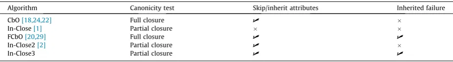
A ‘full closure’ canonicity test to quickly determine repeated concepts[18]. A more efﬁcient, ‘partial closure’, canonicity test[1].

Skipping or inheriting attributes of a parent concept[18,2].

Inheritance of failed canonicity tests[20,29], so that an attribute that has caused a previous failure can be skipped in sub-sequent levels.

The features of the CbO variants described in this article are summarised inTable 1.

5. CbO variants

The following sections present these CbO variants together for the ﬁrst time (including a new variant, In-Close3) and pres-ent them using the same notation, abstraction and style, so that the algorithms and their key features can be clearly iden-tiﬁed and compared.

For the ﬁrst time, each of the variants has been implemented, using the same optimisation, compiler and hardware, to provide a level playing ﬁeld for performance comparisons.

Paper runs of each of the algorithms, using the example context above, are in an on-line appendix[3]. The paper runs are complete, line by line, executions of the algorithms and show that each of the ten concepts,C1toC10, is computed once and

only once by each algorithm. They provide empirical evidence of how each of the algorithms work and allow their key fea-tures to be explored and compared in detail.

5.1. CbO algorithm[18,24,22]

The CbO algorithm of Krajca, Outrata and Vychodil[18]is an efﬁcient realisation of Kuznetsov’s CbO[24,22], where the canonicity test for a new concept is carried out by comparing a newly computed intent,D, with its predecessor,B. If they agree in all attributes up to the current attribute,j, then the new concept is canonical. If, however, there is an attribute in

Dthat is not inBand that comes beforejthen the concept is not canonical (it will have been computed earlier). Thus a new concept is canonical if:

B\Yj¼D\Yj ð3Þ

whereYj is the set of attributes up to but not includingj:

Yj:¼ fy2Yjy<jg ð4Þ

[image:5.544.42.507.625.689.2]

The algorithm also passes the intent of a parent concept down to the next level, so that its attributes can be skipped. In effect this is a simple test to avoid repeatedly closing the parent concept.

Table 1

Comparing the features of the CbO variants.

Algorithm Canonicity test Skip/inherit attributes Inherited failure

CbO[18,24,22] Full closure U

In-Close[1] Partial closure

FCbO[20,29] Full closure U U

In-Close2[2] Partial closure U

(6)

The algorithm is written below as a single procedure calledCompute-ConceptsFrom. The procedure is invoked with the initial conceptðA;BÞ ¼ ðX;X"

Þand initial attributey¼0.

A line-by-line explanation of the algorithm is as follows:

Line 1– Pass conceptðA;BÞto notional procedureProcessConceptto process it in some way (for example, storing it in a set of concepts).

Line 2– Iterate across the context, from starting attributeyup to attributen1.

Line 3– Test if the next attribute is in the current intent,B. If it is, skip it to avoid computing the same concept again.

Line 4– Otherwise, form an extent,C, by intersecting the current extent,A, with the next column of objects in the context.

Line 5– Close the extent to form an intent,D. Thus the conceptðC;DÞis computed (‘fully closed’) before the canonicity test is carried out to determine if it is a new one:

Line 6– Perform the canonicity test by checking that attributes inBandDagree up to the current attribute. If they do then the conceptðC;DÞ, is a new one so:

Line 7– Recursively compute concepts from the new one, starting from the next attribute in the context.

Correctness of CbO– The correctness of the original CbO algorithm is given in[24], and proof of the canonicity test has been shown in[18].

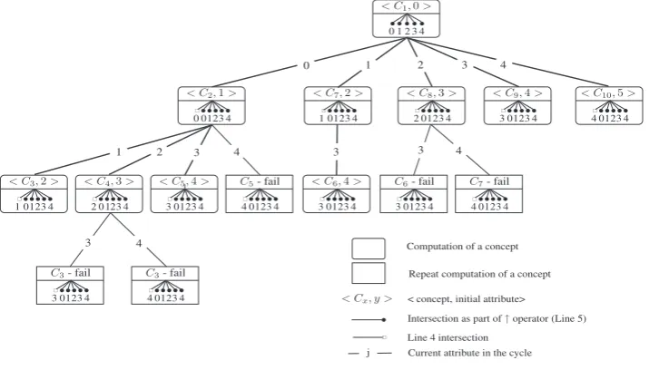
CbO call tree–Fig. 1shows the CbO call tree for the simple example. A rounded box represents the computation of a concept and a square box represents the computation of a repeated concept that then fails the canonicity test. In the upper part of a box, the notationhCx;yirepresents a call to CbO:ComputeConceptsFrom(Cx;yÞ, whereCxis the concept (to be

pro-cessed in Line 1) andyis the initial attribute for the cycle in Line 2. The lower part of a box represents the intersections car-ried out in the computation ofCx. The ‘round headed arrows’ represent intersections carried out by the closure operator". In

the case of the topmost box in the diagram, these intersections are the ones carried out prior to the initial invocation of CbO to compute the initial conceptC1:ðX;X"Þ. In all the other boxes, the intersections are those carried out in computingD C"

in Line 5. An ‘empty square-headed arrow’ represents the intersection carried out in Line 4 to form the extentC. The numbers in the lines connecting the boxes represents the current attribute in the cycle in Line 2.

Thus, for example, the box containinghC2;1ishows the computation ofC2, with the empty square-headed arrow showing

an intersection involving attribute 0 in Line 4:C A\ f0g#and the round-headed arrows showing the subsequent closure intersections in Line 5, involving attributes 0;1;2;3 and 4.

[image:6.544.45.216.84.181.2]

There are a total of 15 closures in the tree, with ﬁve intersections required for each closure, plus 14 extent intersections, making a total of 89 intersections for CbO. A comparative count of closures and intersections for all the algorithms is given in

Table 2.

5.2. In-Close[1]with ‘partial closure’ canonicity test

This section is an updated version of the algorithm given in[1]. In[1]the canonicity test was described as a backtracking approach but here it is realised for the first time as a ‘partial closure’ test. The key difference to the first CbO algorithm above is that the canonicity test is appliedbeforea concept is fully closed. It is sufficient to examine the contextup tothe current attributejto determine its canonicity. For this apartial closureoperator"j_{is defined as a modification of the original closure} operator:

A"j_:_{¼ f}_y₂_Y

jj

8x

2A:xIyg: ð5Þ

The ‘partial closure’ canonicity test determines if the attributes in the intentB, up toj, agree with the attributes in the closure ofCup toj:

(7)

The efﬁciency is thus that a partial closure,C"j_{, is clearly less expensive to compute than a complete closure,}_C"_{. The cost of} the complete closure is a number of intersections equal to the number of attributes,n, whereas the cost of the partial closure is always <n. To calculate the average cost of a partial closure, the average value ofjduring the computation needs to be considered. It is tempting to assume that this average is simplyn=2 but, because a combinatorial order is being followed,

jwill always be the largest value in each combination and it is thus necessary to calculate the average largest value in all combinations. This value is dependent onnand, asnbecomes large, approachesn. Thus the saving is only some fraction ofn, reducing asnincreases. However, in practice there will be a further significant saving since it is sufficient to find a non-canonical attribute only once for the test to fail. Thus the partial closure can be halted as soon as such an attribute is found, turning the test into a linear search from attribute 0 up toj1. This costsðj1Þ=2 for a failed test andj1 for a successful test, approachingn=2 andnrespectively asnbecomes large. Clearly, the failure rate of the canonicity test will depend on the nature of the data. In practice, experiments with data sets[20,29]have shown the failure rate to be typically around 80%, making the average cost of the partial closure test approximately 3n=5, ifnis large. Ifnis small, then the cost can be taken asðn1Þ=2.

Of course, if the canonicity test is passed, new concepts still need to be fully closed and this is carried out incrementally at the next level (hence the algorithm’s name: In(cremental)-Close(ure)), by adding the current attributejto the intentB when-ever the current extentAis found: i.e. wheneverA\ fjg#¼A. The intent is fully closed when the main cycle is completed. Whenever a new concept is detected, the current (not fully closed intent) is passed to the next level so that some parent attributes can be inherited.

The algorithm, shown in In-Close below, is invoked with the initial pairðA;BÞ ¼ ðX;;Þand initial attributey¼0.

Line 2– Form an extent,C, by intersecting the current extent,A, with the next column of objects in the context.

Line 3– If the extent formed,C, equals the extent,A, of the concept whose intent is currently being closed, then. . .

[image:7.544.95.453.55.259.2]

Line 4–. . .add the current attributejto the intent being closed,B.

(8)

Line 6– Otherwise the new partial closure canonicity test is applied. A small simpliﬁcation to the canonicity test can be made becauseBis being completed incrementally withj. In other words, at the time of the test,B¼Bj¼B\Yj. Therefore,

in the canonicity test,B\Yjcan be replaced withB. So if the attributes inBagree with those in the partial closureC"jthe

extent must be a new one so. . .

Line 7– Create a new intentDthat inherits the attributes ofB, plus the current attributej.

Line 8– Pass the new extentC, the partial intentDand the next locationjþ1 to the next level so that concepts from there can be computed and so thatDcan be incrementally closed.

Line 9– Pass conceptðA;BÞto notional procedureProcessConceptto process it in some way (for example, storing it in a set of concepts). Note that in In-Close this happens at the end of the procedure, once the main cycle has completed the closure of the intent,B.

Correctness of In-Close– CbO and In-Close use the same cycle to form the same extents,C. The only pertinent difference up to this point is the skipping of attributes in CbO whenj2B(Line 3). However, this test is only to avoid forming an extent that will fail the canonicity test anyway. Thus to show that In-Close is correct it is sufﬁcient to show that the partial closure canonicity test is equivalent to the original test, in other words, given the same extentC, show that the tests produce the same result:

ðB¼C"j_{Þ ð}_B_\_Y

j¼D\YjÞ

As previously stated, in In-Close the intentBis incrementally closed up to the current attributej, thusB¼B\Yj, so it is

sufﬁcient to show that:

C"j_D_\_Y

j

ReplacingDwithC"_{, from Line 5 of CbO:}

C"j_C"_\_Y

j

Thus, from(1) and (5):

fy2Yjj

8x

2C:xIyg fy2Yj

8x

2C:xIyg \Yj:

So on the left side are all the attributes up tojthat are related to the extent and on the right are all the attributes that are related to the extent, intersected with all the attributes up toj. Both sides are thus clearly equivalent.

In-Close call tree–Fig. 2shows the In-Close call tree for the simple example. As in the CbO call tree, a rounded box rep-resents the computation of a concept and a square box reprep-resents the computation of a repeated concept that then fails the canonicity test. However, a conceptCxnow inherits the intent of the parent concept and has its intent completed as part of

the main cycle. For example, the box withhC2;1ishows the computation of conceptC2. The empty square-headed arrow

shows the intersection involving attribute 0 in Line 2:C A\ f0g#. Attribute 0 is subsequently added toC2’s partial intent

(inherited from its parent conceptC1) in Line 4. In fact,C2’s inherited partial intent was empty since the intent ofC1is empty.

Adding 0 completes the intent ofC2:f0g. There are no intersections involved in the partial closure in Line 6 (no

round-headed arrows) because the partial closure is required only up to, but not including, attribute 0.

Similarly, the box withhC5;4ishows the computation ofC5. Starting the main cycle at attribute 3, the Line 2 intersections

for attributes 3 and 4 result in them both being added to the partial intentf0g, inherited fromC2, thus completing the intent

ofC5:f0;3;4g. The partial closure require to test the canonicity is then up to but not including attribute 3, indicated by the

round-headed arrows.

Altogether there are 59 intersections in the In-Close tree, 30 fewer than for CbO. A full comparative count of closures and intersections is given inTable 2.

5.3. FCbO[20,29]with inherited test failure

In[20,29]a new feature of CbO was added by showing that if the original canonicity test in CbO,B\Yj¼D\Yj, fails for

an attributej R B, then the test will also fail for eachB0

Bwherej R B0_{, as long as}

ððDnBÞ \YjÞcontains an attribute which

[image:8.544.36.509.74.137.2]

is not inB0. This information can be passed from one level to the next by recording the intentDcomputed before a failed

Table 2

Comparison of closures and intersections for the simple context example.

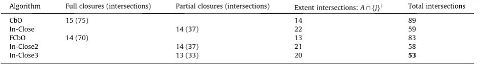
Algorithm Full closures (intersections) Partial closures (intersections) Extent intersections:A\ fjg# _{Total intersections}

CbO 15 (75) 14 89

In-Close 14 (37) 22 59

FCbO 14 (70) 13 83

In-Close2 14 (37) 21 58

(9)

canonicity test for an attributej. If this record is denoted byNj_{, then if}_B

\Yj¼D\Yjfails thenNj¼D.Ns for each attribute

are passed to the next level as inherited test failures. For a particular attributej, if there is an attribute inNj_before_j_{that is}

not inBbeforej, then there is no need to carry out the original canonicity test.

To obtain all the failed intents, before passing them to the next level, a combined breadth-ﬁrst, depth-ﬁrst approach is used. All attributes are iterated and tested for failure before going to the next level. New concepts, as they are found, are stored in a queue for later processing. Once all attributes have been iterated in the main cycle, the stored concepts are pro-cessed by calling the algorithm recursively and passing the corresponding set of failed intents to the next level.

The algorithm is given below. It is invoked with the initial conceptðA;BÞ ¼ ðX;X"

Þ, initial attributey¼0 and a set of emptyNs,fNy_{¼ ;j}_y₂_Y_g_.

Line 2– Iterate across the context (breadth-ﬁrst), from starting attributeyup to attributen1.

Line 3– The record of failure for attributej,Mj, to be inherited by the next level, is set to the current record of failureNj.

Line 4– Skip attributes inBand those that have an inherited record of failure.

Line 6– Close the extent to form an intent,D.

Line 7– Perform the original canonicity test.

[image:9.544.95.452.55.258.2]

Line 8– If the concept is a new one, store it in a queue along with the attribute it was computed at.

(10)

Line 10– Otherwise set the record of failure for attributej;Mj, to the intent that failed the canonicity test.

Line 11– Now do the depth-ﬁrst part by getting each stored concept from the queue. . .

Line 12– and passing it to the next level, along with the stored starting attribute for the next level and the records of failure from this level.

Correctness of FCbO– The correctness of FCbO and proof of the inheritance of canonicity failure is given in[20,29].

FCbO call tree–Fig. 3shows the call tree for FCbO. It is the same as the tree for CbO except that a repeat computation of conceptC3is avoided because of an inherited canonicity failure. The inherited failure is from the ﬁrstC3canonicity test

fail-ure which occurred after the computation ofC4(see the listing of the paper run of FCbO for a line by line demonstration of

the inherited failure[3]). This gives a saving of six intersections compared to CbO. A comparative count of closures and inter-sections is given inTable 2.

5.4. In-Close2[2]with ‘partial closure’ test and fully inherited intents

The algorithm presented here is an updated version of that presented in[2]. In-Close2 has been ‘bred’ from In-Close and FCbO to combine the efficiencies of the partial closure canonicity test with full inheritance of the parent intent. It achieves this by adapting and adopting the breadth-first and depth-first approach of FCbO[20,29]. The main cycle is completed before passing to the next level, so that all the attributes of a parent intent can be passed down to the next level rather than just some of them. Like In-Close, child intents only have to be ‘finished off’ by adding attributes whenA¼C, but now additional attributes afterjare also inherited and can be skipped. During the main cycle, whilst the current intent is being closed, new extents that pass the canonicity test are stored in a queue, similar to the queue in FCbO, to be processed after the main cycle has completed.

The In-Close2 algorithm, given below, is invoked the same way as In-Close, with an initialðA;BÞ ¼ ðX;;Þand initial attri-butey¼0.

Line 2– Skip attributes already inB. Because intents now inherit all of their parent’s attributes, these can be skipped.

Line 3– Form an extent,C, by intersecting the current extent,A, with the next column of objects in the context.

Line 7– Otherwise, test the canonicity. Theunsimpliﬁedversion of the partial closure test(6)is now used because intents now contain inherited attributes afterj.

Line 8– If the canonicity test is passed, place the new extent,C, and the location where it was found,j, in a queue for later processing.

Lines 10– The queue is processed by obtaining each new extent and associated location from the queue.

Line 11– Each new partial intent,D, inherits all the attributes from its completed parent intent,B, along with the attribute,

j, where its extent was found.

(11)

Correctness of In-Close2– The process of incremental closure and canonicity testing (lines 3–7) is unchanged from CbO version 2, apart from the new initial testj R B. To show that CbO version 3 is correct it is thus sufﬁcient to show that the new test does not exclude any required attributes from this process. The possible outcomes after formingCare either adding the attribute toBinB B[ fjgor carrying out the canonicity testB\Yj¼C"j. It is thus necessary to show that any attributes

excluded by the test (by failingj R B) do not affect these outcomes.

For the ﬁrst outcome, ifj2BthenB B[ fjg ¼B. In other words,jis already inB, so adding it would have no effect. For the second outcome, ifj2BthenB\Yjwould be unchanged sinceYjby deﬁnition does not includej.

Thus it is not possible for the new test to exclude any required attributes from the computation.

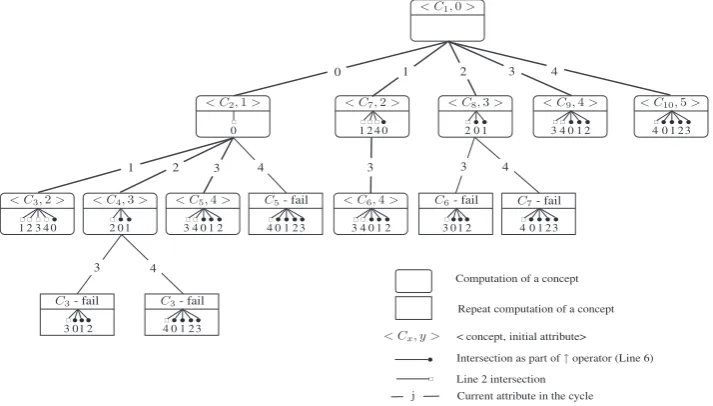
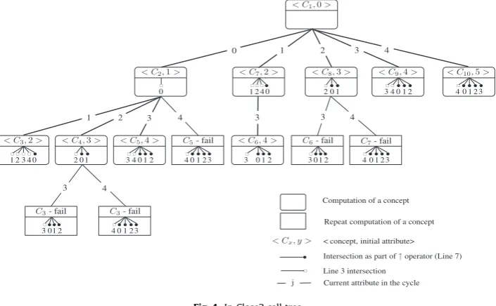
In-Close2 call tree–Fig. 4shows the call tree for In-Close2. It is the same as the tree for In-Close except that now concept

C6inherits an additional attribute, 4, from conceptC7. This is because the main cycle is now completed before passing to the

next level, so that attribute 4 is added to the parent intent before the next level is invoked. Thus one intersection is saved compared to In-Close. A comparative count of closures and intersections is given inTable 2.

5.5. In-Close3 with ‘partial closure’ test, inherited intents and inherited failure test

This is a new variant of CbO that ‘breeds’ In-Close2 and FCbO to include the partial closure canonicity test and the full inheritance of intents of In-Close2, along with the inherited failed canonicity tests of FCbO.

[image:11.544.94.451.54.275.2]

The In-Close3 algorithm is given below.

(12)

Line 1– Iterate across the context (breadth-ﬁrst), from starting attributeyup to attributen1.

Line 2– The record of failure for attributej,Mj, to be inherited by the next level, is set to the current record of failureNj.

Line 3– Skip attributes already inBand those that have an inherited record of failure.

Line 8– Otherwise, perform the partial closure canonicity test and, if the extent is new. . .

Line 9–. . .store it in a queue along with the attribute it was computed at.

Line 11– Otherwise set the record of failure for attributej;Mj, to the intent that failed the canonicity test.

Line 11– Now do the depth-ﬁrst part by getting each stored concept from the queue. . .

Line 11– and passing it to the next level, along with the stored starting attribute for the next level and the records of failure from this level.

Line 11– if the partial closure canonicity test fails for an attributej, the attributes in the partial closure are recorded byMj.

Lines 13– The queue is processed by obtaining each new extent and associated location from the queue.

Line 14– Each new partial intent,D, inherits all the attributes from its completed parent intent,B, along with the attribute,

j, where its extent was found.

Line 15– CallComputeConceptsFromto compute child concepts fromjþ1 and to complete the intent,D, also passing down the records of failure from this level.

Correctness of In-Close3– The correctness of the canonicity test has been shown above as has the completeness of the closure. However, the record of failure in In-Close3 isMj C"j_{whereas in FCbO it is}_Mj _D_¼_C"_{. Thus it must be shown that} the records are equivalent in the inherited canonicity failure testNj

\Yj#B\Yj.

SinceC"

\Yj¼C"j, then for In-Close3,Nj\Yj¼C"\Yj\Yj¼C"\Yj, which is the test for FCbO. Thus the two tests are

equivalent.

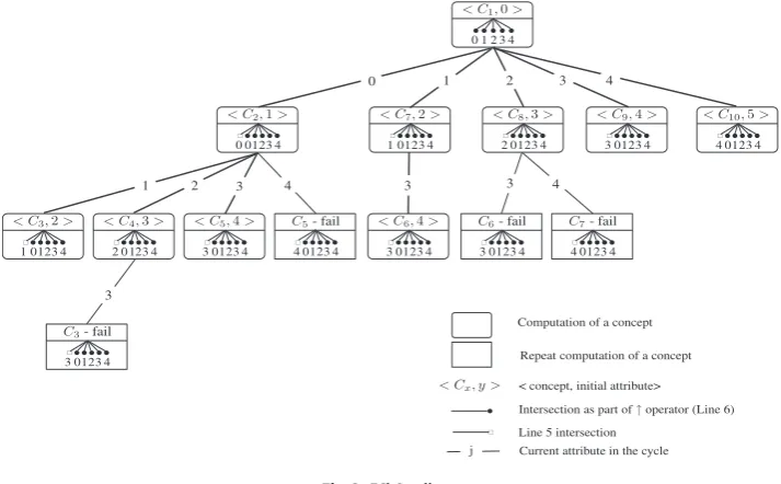
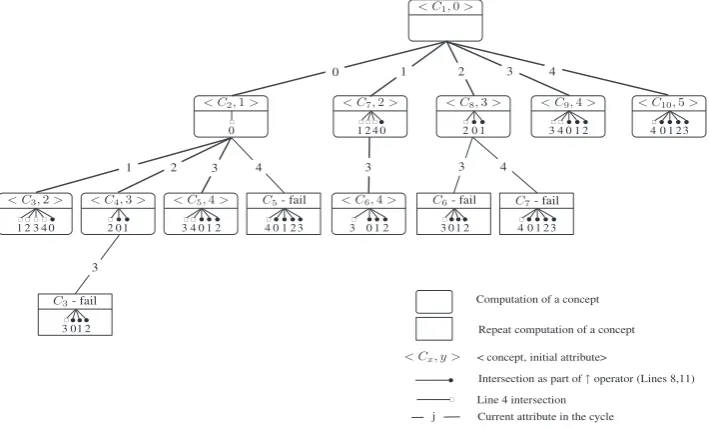
In-Close3 call tree–Fig. 5shows the call tree for In-Close3. It is the same as the tree for In-Close2 except that now the second repeat ofC3is avoided, as it was with FCbO. The ﬁrst canonicity failure ofC3is inherited during the computation of

C4. Thus, a saving of ﬁve intersections is made compared to In-Close2. A comparative count of closures and intersections is

given inTable 2.

6. Performance evaluation

6.1. Paper runs using the simple example

Table 2compares the performance of each algorithm using the simple context example from Section2. The table counts

[image:12.544.93.446.55.273.2]

and compares the number of full and partial closures and the number of extent intersections,A\ fjg#. Because closure itself involves repeated intersections of an extent with columns of the context, it is convenient to use the intersection as a measure

(13)

of performance. For a full closure,C"_{, there are}_n_{intersections (in the example,}_n_¼_{5) and for a partial closure,}_C"j_{, there are}

j1 intersections. To perform the evaluation, a paper run of each algorithm was carried out, line by line. These are too lengthy to be presented here but are available as an on-line appendix[3].

In-Close requires one less closure than CbO. This is because CbO (and FCbO) require an initial closure,X"_{, that In-Close,}

and subsequent In-Close variants, do not. The partial closure test saves 38 intersections for In-Close, compared to the full closures in CbO. In-Close, however, requires an additional 8 extent intersections to complete the closure of intents. Thus overall, In-Close required 30 fewer intersections than CbO. FCbO saved six intersections compared to CbO through inherited failure avoiding a repeated concept computation. In-Close2 saved an intersection compared to In-Close by inheriting an attri-bute in a parent intent. In-Close3 saved a further ﬁve intersections through inherited canonicity failure.

6.2. Implementations

Each algorithm was been implemented in C++ and a series of tests were carried out using contexts created from real data sets, artiﬁcial data sets and randomised data sets. The experiments were carried out using a standard Windows PC with an Intel E4600 2.39 GHz processor and 3 GB of RAM. The times for the programs include data pre-processing, such as sorting, but exclude administrative aspects, such as data ﬁle input.

To create a level playing ﬁeld for testing, the algorithms were implemented with the same two optimisations. Although it would have been possible to create un-optimised implementations, times for real data sets would be prohibitively slow and comparisons with times presented elsewhere for similar experiments would be unhelpful. The two optimisations used were:

Sorting context columns in order of density Implementing the context as a bit-array

The practice of column-sorting to improve concept computation is well known[9]. By doing so, there are fewer canonicity test failures. This is because there is less chance of ﬁndingAbefore attributejsince the context is less dense before attribute

j.

The use of bit-arrays is well known in computation, allowing a SIMD (Single Operation – Multiple Data) approach, where, for example, 32 context rows can be intersected simultaneously using standard 32-bit operations[18].

For the In-Close variants, the full savings of the partial closure canonicity test were realised in the implementations: for the test to fail it is only necessary to ﬁnd one attribute that is not canonical. Thus the partial closure test can be ended as soon as such an attribute is found, even if that is beforej1.

The inherited canonicity failure required the creation of a two-dimensional array to implement the set of failure records, fNy

[image:13.544.96.451.55.269.2]

jy2Yg, one failed intent for each attribute. This was required to be passed to each level of recursion. Although the use of pointers reduces the need for copying arrays in memory, the manipulation and accessing of the arrays gives rise to some additional complexity in the computation.

(14)

Extents were stored as ‘end-to-end’ lists of integers in a one-dimensional array to save memory. Storing extents in a two-dimensional array may, in theory, give rise to some time savings, being a simpler data structure. However, in practice, with typical data sets, the large number of objects and concepts makes the required size of the array prohibitive.

Intents were stored in a two-dimensional bit-array, each being stored asnbits. The use of bits and the fact that the num-ber of attributes is typically much smaller than objects, makes the memory requirements tractable. For testingj R B, the Boolean nature of the bit-array version of intents is an efﬁcient structure, with the test becoming:if not(B[j]).

For carrying out the extent intersection,C A\ fjg#, it was a simple case of testing the bit-position in columnjof the context for each integer inA. For the In-Close variants, the size ofC(produced as a by-product of the extent intersection) was used to test equality betweenCandA. In effect the test becomes:jAj ¼ jCj, incurring no additional overhead.

For the closure/partial closure ofC, a bit-wise Booleanandoperator was used to ‘parse’ 32 columns of the context at a time, using the integers inAto identify the rows to test. For the In-Close variants, of course, as soon asCwas found in a col-umn beforejand not inB, the closure was halted.

6.2.1. Real data set experiments

[image:14.544.36.503.325.412.2]

Three of the data sets are from the UCI Machine Learning Repository[11]:Mushroom,AdultandInternet Ads. A fourth data set,Student, is a set of results from a student questionnaire used to obtain course feedback at Sheffield Hallam University, UK in 2010. The data sets provide a range of size and density to test the implementations under a variety of real conditions. Formal contexts were created from these data sets using well known FCA scaling techniques where many-valued data is converted into Boolean form[33,13,6]. The results are given inTable 3. The results bear out the analysis and comparison of the algorithms given earlier, showing that the partial closure canonicity test is a significant factor in the efficiency of the implementations of the algorithms, but also indicate that attribute inheritance/skipping and inherited canonicity test failure contribute to time savings.

Table 3

Real data set results (timings in seconds).

Mushroom Adult Internet Ads Student

jGj jMj 8;124125 32;561124 3;2791;565 587145

Density 17.36% 11.29% 0.97% 24.50%

#Concepts 226,921 1,388,469 16,570 22,760,243

CbO 0.66 3.06 0.56 32.68

In-Close 0.40 1.65 0.12 11.42

FCbO 0.35 2.06 0.21 17.20

In-Close2 0.35 1.48 0.08 9.89

In-Close3 0.29 1.62 0.10 9.38

Table 4

Comparison of closures and intersections for the real data sets.

Full/partial closures (intersections) Extent intersections Total intersections

Adult

CbO 300,674 (37,283,576) 300,673 37,584,249

InClose 300,673 (26,994,788) 356,967 27,351,755

FCbO 153,745 (19,064,380) 153,745 19,218,125

InClose-II 300,673 (26,994,788) 331,267 27,326,055

InClose-III 153,745 (13,834,074) 184,339 14,018,413

Ad

CbO 1,867,690 (2,922,934,850) 1,867,689 2,924,802,539

InClose 1,867,689 (2,190,704,598) 1,924,704 2,192,629,302

FCbO 333,626 (522,124,690) 333,626 522,458,316

InClose-II 1,867,689 (2,190,704,598) 1,897,257 2,192,601,855

InClose-III 333,626 (386,500,353) 363,194 386,863,547

Mushroom

CbO 1,164,839 (145,604,875) 1,164,838 146,769,713

InClose 1,164,838 (129,543,924) 2,727,529 132,271,453

FCbO 282,165 (35,270,625) 282,165 35,552,790

InClose-II 1,164,838 (129,543,924) 1,191,891 130,735,815

InClose-III 282,164 (31,386,369) 309,217 31,695,586

Student

CbO 55,038,423 (7,980,571,335) 55,038,422 8,035,609,757

InClose 55,038,422 (7,632,184,009) 78,630,232 7,710,814,241

FCbO 33,003,581 (4,785,519,245) 33,003,581 4,818,522,826

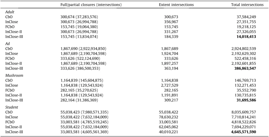
[image:14.544.36.504.451.689.2]

(15)

The programs were then instrumented to count the number of closures and intersections carried out (seeTable 4) to com-pare the number of these operations with the timings. The ranking of algorithms is similar except for FCbO which is now second best after In-Close3, in terms of fewest intersections. It is clear that, in practice, there is higher number of inherited canonicity failures than that shown in the simple example. Thus, the most striking difference is in the large savings of clo-sures made by the inherited failure tests of FCbO and In-Close3, significantly reducing the number of intersections required. However, the savings in time are not proportionate to the savings in intersections. It would seem that the overheads of the additional computational complexity of inherited failure were having a significant impact on the performance of these implementations, even though efficient coding was used. Similar results have been obtained elsewhere[30,17,29].

6.2.2. Artiﬁcial data set experiments

The following artiﬁcial data sets were used:

M7X10G120K – a data set based on simulating many-valued attributes. The scaling of many-valued attributes is simu-lated by creating ‘blocks’ in the context containing disjoint columns. There are 7 blocks, each containing 10 disjoint col-umns. The data set was created by writing a simple C++ program with a random number generator.

M10X30G120K – a similar data set, this time with a context containing 10 blocks, each with 30 disjoint columns. T10I4D100K – an artiﬁcial data set from the FIMI data set repository[15].

[image:15.544.39.508.304.392.2]

The results of the artiﬁcial data set experiments are given inTable 5. The results tend to replicate the ﬁndings of the real data set experiments and corroborate the previous comparison of the algorithms.

Table 5

Artiﬁcial data set results (timings in seconds). Figures in bold are the fastest times.

M7X10G120K M10X30G120K T10I4D100K

jGj jMj 120;00070 120;000300 100;0001;000

Density 10.00% 3.33% 1.01%

#Concepts 1,166,343 4,570,498 2,347,376

CbO 2.51 31.26 49.45

In-Close 1.26 18.95 16.02

FCbO 1.67 22.33 29.41

In-Close2 1.21 12.10 11.23

[image:15.544.165.381.386.528.2]

In-Close3 1.39 10.42 11.04

[image:15.544.171.381.564.674.2]

Fig. 6.Comparison of performance with varying number of attributes. 5% density, 5000 objects. #Concepts range from approx. 1,000,000–22,000,000.

(16)

6.2.3. Random data set experiments

Three series of random data experiments were carried out to compare the performance of In-Close2 and FCbO, testing the affect of changes in the number of attributes, context density, and number of objects. Note that randomly assigning crosses in a table gives rise to a much larger number of concepts compared to real data sets of similar size and density.

Attributes series– with 5% density and 5000 objects, the number of attributes was varied between 300 and 1000 (Fig. 6). The number of concepts varied from approximately 1 million to 22 million.

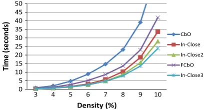
Density series– with 200 attributes and 10,000 objects, the density of 1s in the context was varied between 3% and 10%

(Fig. 7). The number of concepts varied from approximately 200 thousand to 19 million.

Objects series– with 5% density and 200 attributes, the number of objects was varied between 30,000 and 100,000 (Fig. 8). The number of concepts varied from approximately 4 million to 22 million.

The results of randomised data set series also tend to bear out the analysis and comparison of the algorithms given earlier, showing the partial closure canonicity test to be the most signiﬁcant factor in the efﬁciency of the algorithms, but again also indicating that attribute inheritance/skipping and inherited canonicity test failure add to time savings. This is particularly clear in the comparison of In-Close and In-Close2 with respect to FCbO. In the density series, where one might expect a high degree of inheritance, FCbO does better than In-Close, but not In-Close2 which ‘bred’ the inheritance from FCbO. In the case of the attribute and density series, In-Close3 performed best, but in the object series In-Close2 was slightly quicker. Both versions incorporate the partial closure test and skip inherited attributes but In-Close3 has the inherited canonicity test fail-ure, ‘bred’ from FCbO, whereas In-Close2 does not. Again it seems that the complexity overhead of maintaining the records of failure balances the savings in intersections, particularly where the number of objects increases.

7. Conclusions and further work

The analysis and comparison of the CbO algorithms presented here, and the results of the experiments carried out, show that the partial closure canonicity test is the most significant factor in the efficiency of CbO algorithms. However, in terms of the number of closures required, the inherited test failure approach of FCbO is the most significant. Breeding In-Close with FCbO, to create In-Close2, incorporating attribute inheritance with partial closure, produced a significant improvement in efficiency, resulting from a significant increase in attributes skipped. Further breeding with FCbO to create In-Close3, incor-porating inherited canonicity failure, produced an algorithm that usually, but not always, performed slightly better than In-Close2. It is debatable, therefore, which of In-Close2 and In-Close3 is the ‘best of breed’. Although inherited failure made a significant difference to CbO, it had much less impact on In-Close2. Although there were far fewer intersections when inher-ited failure was incorporated, this appeared to be masked by the extra time taken with the inherinher-ited failure mechanisms. In case this was due to an inefficient implementation by the author, the source code provided by the original authors of FCbO was also timed, with the same results. Whilst it is hard to instrument the inherited failure mechanisms directly, as much is to do with memory use and the associated code is rather dispersed, it was possible, by removing all parts involved with inher-ited failure and the associated structures, to compare FCbO and In-CloseIII, with and without the feature. This experiment confirmed the timings: although there was a large increase in closures with the parts removed, there was only comparatively small slowdown in the overall computation. Thus it is questionable that the added complexity of inherited failure feature provides enough benefit to the performance of these algorithms to make it worthwhile. However, the large reduction in clo-sures resulting from inherited failure does make further work in this area tempting. Can an algorithm be found that incor-porates this feature of inherited canonicity failure but without the current complexity?

Future work is also required in increasing performance through parallel processing. Work has been carried out to develop parallel versions of CbO (PCbO) and FCbO (PFCbO)[18,20]but not as yet for the In-Close variants.

[image:16.544.169.376.54.170.2]

Besides work on further improving the efﬁciency of the computation of formal concepts, what is also required is the development of more applications that harness this power, such as in the areas of classiﬁcation and machine learning. These

(17)

improvements in efﬁciency make FCA available to a larger scale of data, but new tools and techniques are required to provide useful and meaningful results from the large numbers of concepts typically produced by such computations.

Implementations of these algorithms (In-Close variants and FCbO) are available open-source atSourceForge[4,19].

Acknowledgments

This work is part of the CUBIST project (‘‘Combining and Uniting Business Intelligence with Semantic Technologies’’), funded by the European Commission’s 7th Framework Programme of ICT, under topic 4.3: Intelligent Information Manage-ment. Project ID: CUBIST-257403.

Appendix A. Supplementary material

Supplementary data associated with this article can be found, in the online version, at http://dx.doi.org/10.1016/

j.ins.2014.10.011.

References

[1] S. Andrews, In-close, a fast algorithm for computing formal concepts, in: S. Rudolph, F. Dau, S.O. Kuznetsov, (Eds.), ICCS 2009, CEUR WS, vol. 483, 2009. <http://sunsite.informatik.rwth-aachen.de/Publications/CEUR-WS/Vol-483/>.

[2]S. Andrews, In-close2, a high performance formal concept miner, in: S. Andrews, S. Polovina, R. Hill, B. Akhgar (Eds.), Conceptual Structures for Discovering Knowledge – Proceedings of the 19th International Conference on Conceptual Structures (ICCS), Springer, 2011, pp. 50–62.

[3] S. Andrews, Appendix to a Best of Breed Approach to Designing a Fast Algorithm for Computing Fixpoints of Galois Connections, 2013. <https:// dl.dropboxusercontent.com/u/3318140/bob_appendix.pdf>.

[4] S. Andrews, In-Close Program, 2013. <http://sourceforge.net/projects/inclose/>.

[5] S. Andrews, C. Orphanides, Analysis of large data sets using formal concept lattices, in:[21], 2010, pp. 104–115.

[6]S. Andrews, C. Orphanides, Fcabedrock, a formal context creator, in: M. Croitoru, S. Ferre, D. Lukose (Eds.), ICCS 2010, LNCS, vol. 6208/2010, Springer, 2010.

[7] D. Borchman, A generalized next-closure algorithm – enumerating semilattice elements from a generating set, in: L. Szathmary, U. Priss, (Eds.), Proceedings of Concept Lattices and thie Applications (CLA) 2012, Universidad de Malaga, 2012, pp. 9–20.

[8]J.P. Bordat, Calcul pratique du treillis de Galois dune correspondance, Math. Sci. Hum. 96 (1986) 31–47. [9]C. Carpineto, G. Romano, Concept Data Analysis: Theory and Applications, J. Wiley, 2004.

[10]M. Chein, Algorithme de recherche des sous-matrices premires dune matrice, Bull. Math. Soc. Sci. Math. R.S. Roumanie 13 (1969) 21–25. [11] A. Frank, A. Asuncion, UCI Machine Learning Repository, 2010. <http://archive.ics.uci.edu/ml>.

[12] B. Ganter, Two Basic Algorithms in Concept Analysis, FB4-Preprint 831, TH Darmstadt, 1984. [13]B. Ganter, R. Wille, Formal Concept Analysis: Mathematical Foundations, Springer-Verlag, 1998.

[14]R. Godin, R. Missaoui, H. Alaoui, Incremental concept formation algorithms based on Galois lattices, Comput. Intell. 11 (2) (1995) 246–267. [15] B. Goethals, Frequent Itemset Implementations (fimi) Repository, 2010. <http://fimi.cs.helsinki.fi/>.

[16]M. Kaytoue, S.O. Kuznetsov, A. Napoli, S. Duplessis, Mining gene expression data with pattern structures in formal concept analysis, Inf. Sci. 181 (10) (2011) 1989–2001.

[17]M. Kirchberg, E. Leonardi, Y.S. Tan, S. Link, R.K.L. Ko, B.S. Lee, Formal concept discovery in semantic web data, LNAI, vol. 7278, Springer-Verlag, Berlin Heidelberg, 2012.

[18] P. Krajca, J. Outrata, V. Vychodil, Parallel recursive algorithm for FCA, in: R. Belohavlek, S. Kuznetsov, (Eds.), Proceedings of Concept Lattices and their Applications, 2008.

[19] P. Krajca, J. Outrata, V. Vychodil, FCbO Program, 2012. <http://fcalgs.sourceforge.net/>.

[20] P. Krajca, V. Vychodil, J. Outrata, Advances in Algorithms Based on CbO, In:[21], 2010, pp. 325–337.

[21] M. Kryszkiewicz, S. Obiedkov, (Eds.), Proceeding of 7th International Conference on Concept Lattices and Their Applications, CLA 2010, Seville, University of Sevilla, 2010.

[22]S. Kuznetsov, Learning of simple conceptual graphs from positive and negative examples, in: J. Zytkow, J. Rauch (Eds.), PKDD’99, Lecture Notes in Computer Science, vol. 1704, Springer, 1999, pp. 384–391.

[23]S. Kuznetsov, S. Obiedkov, Comparing performance of algorithms for generating concept lattices, J. Exp. Theor. Artif. Intell. 14 (2002) 189–216. [24]S.O. Kuznetsov, Mathematical aspects of concept analysis, Math. Sci. 80 (2) (1996) 1654–1698.

[25]S.O. Kuznetsov, On computing the size of a lattice and related decision problems, Order 18 (4) (2001) 313–321.

[26]C. Lindig, Fast concept analysis, in: Working with Conceptual Structures: Contributions to ICCS 2000, Shaker Verlag, Aachen, 2000, pp. 152–161. [27]E. Norris, Maximal rectangular relations, in: Proceedings of the 1st Conference on Fundamentals of Computing Theory, Lecture Notes in Computer

Science, vol. 56, Springer, 1977, pp. 476–481.

[28]L. Nourine, O. Raynaud, A fast algorithm for building lattices, Inf. Process. Lett. 71 (1999) 199–204.

[29]J. Outrata, V. Vychodil, Fast algorithm for computing ﬁxpoints of Galois connections induced by object-attribute relational data, Inf. Sci. 185 (1) (2012) 114–127.

[30] F. Strok, A. Neznanov, Comparing and analyzing the computational complexity of fca algorithms, in: Proceedings of the 2010 Annual Research Conference of the South African Institute of Computer Scientists and Information Technologists, 2010, pp. 417–420.

[31]T. Tanabata, K. Sawase, H. Nobuhara, B. Bede, Interactive data mining for image databases based on FCA, J. Adv. Comput. Intell. Intell. Inf. 14 (3) (2010) 303–308.

[32]D. Van der Merwe, S. Obiedkov, D. Kourie, Addintent: a new incremental algorithm for constructing concept lattices, in: P. Eklund (Ed.), ICFCA 2004, Lecture Notes in Computer Science, vol. 2961, Springer, 2004, pp. 372–385.

[33]K.E. Wolff, A ﬁrst course in formal concept analysis: how to understand line diagrams, Adv. Stat. Software 4 (1993) 429–438.

(18)