A comparison of stiffness analysis methods for robotic systems

GONÇALVES, Rogério Sales, CARBONE, Giuseppe

<http://orcid.org/0000-0003-0831-8358>, CARVALHO, João Carlos Mendes and CECCARELLI,

Marco

Available from Sheffield Hallam University Research Archive (SHURA) at:

http://shura.shu.ac.uk/14380/

This document is the author deposited version. You are advised to consult the

publisher's version if you wish to cite from it.

Published version

GONÇALVES, Rogério Sales, CARBONE, Giuseppe, CARVALHO, João Carlos

Mendes and CECCARELLI, Marco (2016). A comparison of stiffness analysis

methods for robotic systems. International journal of mechanics and control, 17 (2),

35-58.

Copyright and re-use policy

See

http://shura.shu.ac.uk/information.html

International Journal

of

Mechanics and Control

Editor: Andrea Manuello Bertetto

Scopus Indexed Journal

Reference Journal of IFToMM Italy International Federation for the Promotion of Mechanism and Machine Science

Y0

X0

O0

a

q, b

Vs

Published by Levrotto&Bella – Torino – Italy E.C.

Honorary editors

Guido Belforte Kazy Yamafuji

Editor: Andrea Manuello Bertetto

General Secretariat: Matteo D. L. Dalla Vedova

Atlas Akhmetzyanov

V.A. Trapeznikov Institute of Control Sciences of Russian Academy of Sciences

Moscow – Russia

Domenico Appendino Prima Industrie Torino – Italy

Kenji Araki Saitama University Saitama – Japan

Guido Belforte Politecnico di Torino Torino – Italy

Bruno A. Boley Columbia University, New York – USA

Elvio Bonisoli Politecnico di Torino Torino – Italy

Marco Ceccarelli

LARM at DIMSAT, University of Cassino Cassino – Italy

Amalia Ercoli Finzi Politecnico di Milano Milano – Italy

Carlo Ferraresi Politecnico di Torino Torino – Italy

Anindya Ghoshal Arizona State University Tempe – Arizona – USA

Nunziatino Gualtieri

Space System Group, Alenia Spazio Torino – Italy

Alexandre Ivanov Politecnico di Torino Torino – Italy

Giovanni Jacazio Politecnico di Torino Torino – Italy

Takashi Kawamura Shinshu University Nagano – Japan

Kin Huat Low

School of Mechanical and Aerospace Engineering Nanyang Technological University

Singapore

Paolo Maggiore Politecnico di Torino Torino – Italy

Andrea Manuello Bertetto University of Cagliari Cagliari – Italy

Stamos Papastergiou Jet Joint Undertaking Abingdon – United Kingdom

Mihailo Ristic Imperial College

London – United Kingdom

Jànos Somlò

Technical University of Budapast Budapest – Ungary

Jozef Suchy

Faculty of Natural Science Banska Bystrica – Slovakia

Federico Thomas

Instituto de Robótica e Informática Industrial Barcelona – Espana

Furio Vatta

Politecnico di Torino Torino – Italy

Vladimir Viktorov Politecnico di Torino Torino – Italy

Kazy Yamafuji

University of Electro-Communications Tokyo – Japan

Official Torino Italy Court Registration n.5390, 5th _{May 2000}

Deposito presso il Tribunale di Torino numero 5390 del 5 maggio 2000 Direttore responsabile:

Editor:

Andrea Manuello Bertetto

Honorary editors:

Guido Belforte

General Secretariat:

Matteo D. L. Dalla Vedova

Kazy Yamafuji

The Journal is addressed to scientists and engineers who work in the fields of mechanics (mechanics, machines, systems, control, structures). It is edited in Turin (Northern Italy) by Levrotto&Bella Co., with an international board of editors. It will have not advertising.

Turin has a great and long tradition in mechanics and automation of mechanical systems. The journal would will to satisfy the needs of young research workers of having their work published on a qualified paper in a short time, and of the public need to read the results of researches as fast as possible.

Interested parties will be University Departments, Private or Public Research Centres, Innovative Industries.

Aims and scope

The International Journal of Mechanics and Control publishes as rapidly as possible manuscripts of high standards. It aims at providing a fast means of exchange of ideas among workers in Mechanics, at offering an effective method of bringing new results quickly to the public and at establishing an informal vehicle for the discussion of ideas that may still in the formative stages.

Language: English

International Journal of Mechanics and Control will publish both scientific and applied contributions. The scope of the journal includes theoretical and computational methods, their applications and experimental procedures used to validate the theoretical foundations. The research reported in the journal will address the issues of new formulations, solution, algorithms, computational efficiency, analytical and computational kinematics synthesis, system dynamics, structures, flexibility effects, control, optimisation, real-time simulation, reliability and durability. Fields such as vehicle dynamics, aerospace technology, robotics and mechatronics, machine dynamics, crashworthiness, biomechanics, computer graphics, or system identification are also covered by the journal.

Please address contributions to

Prof. Andrea Manuello Bertetto PhD Eng. Matteo D. L. Dalla Vedova

Dept. of Mechanical and Aerospace Engineering Politecnico di Torino

C.so Duca degli Abruzzi, 24. 10129 - Torino - Italy - E.C.

www.jomac.it

e_mail: [email protected]

Subscription information

Subscription order must be sent to the publisher:

Libreria Editrice Universitaria Levrotto&Bella

C.so Luigi Einaudi 57/c – 10129 Torino – Italy

www.levrotto-bella.net

A COMPARISON OF STIFFNESS ANALYSIS METHODS FOR

ROBOTIC SYSTEMS

Rogério Sales Gonçalves*, Giuseppe Carbone**, João Carlos Mendes Carvalho*, Marco Ceccarelli**

* School of Mechanical Engineering, Federal University of Uberlandia, Uberlandia / MG, Brazil

** LARM, DiMSAT, University of Cassino and South Latium, Cassino, Italy

ABSTRACT

A robotic structure consists of a kinematic chain composed by links that can be rigid or flexible, interconnected by joints. One of the outstanding problems in robotic design and operation is to estimate a robot behavior under the action of external loads. In particular, it is needed a standard procedure to obtain the stiffness performance through the whole robot workspace. This paper presents a review about the main available methods to calculate the robotic systems stiffness performance in terms of a local Cartesian stiffness matrix. Specific attention is addressed to methods based on lumped parameters both by using the kinematic and dynamic forces distributions and by using Jacobian matrices. This paper also describes methods based on matrix structural analysis (MSA) and finite element analysis (FEA). Two cases of study have been reported to analyze and compare the above mentioned methodologies for providing a suitable mean to choose the most appropriate method for a given application.

Keywords: stiffness analysis, compliant displacements, matrix structural analysis, jacobian matrix, FEA

1 INTRODUCTION

A robotic structure is based on a kinematic chain composed by links that can be rigid or flexible and are interconnected by joints. One of the open issues in Robotics is to determine the stiffness performance of a robot within a standard procedure although several different stiffness analysis methods are available in a wide literature. Stiffness can be defined as the capacity of a mechanical system to sustain loads without excessive changes of its geometry, which are known as deformations or compliant displacements [1]. Compliant displacements produce negative effects on static behavior, fatigue strength, wear resistance, efficiency (friction losses), accuracy and dynamic stability (vibration), [1-4]. The growing importance of high accuracy and dynamic performance for robots, both with serial and parallel structures, has increased the use of high strength materials and lightweight designs achieving significant reduction of cross-sections and weight.

Contact author: Rogério Sales Gonçalves1

1

Av. João Naves de Ávila, 2121 - Campus Santa Mônica - Uberlândia - MG - CEP 38400-902, Brazil.

E-mail: [email protected]

Nevertheless, these solutions also increase structural deformations and may result in intense resonance and self-excited vibrations at high speed [1]. Therefore, the study of the stiffness becomes of fundamental importance for the design of a robotic structure in order to properly choose materials, component geometry, shape and size, and interaction of each component with others.

The overall stiffness of a robot depends on several factors such as the size and material used for links, the mechanical transmission mechanisms, actuators and the controller dynamics as described, for example in [2]. In general, to achieve a high stiffness performance, many parts should be large and heavy. However, to obtain high speed motions most of the parts should be small and light. Additionally, the robot stiffness is greatly affected by robot configuration as reported for example in [3].

compliant displacements ∆∆∆∆x occurring to a frame fixed at the end of the kinematic chain when a wrench ∆∆∆∆F acts upon the mechanism structure. If necessary, compliant displacements of intermediate elements of the structure can be obtained too. It is to note that a stiffness matrix is obtained as function of the configuration. Thus, one stiffness matrix has to be calculated at each robot configuration. Then, it is also necessary to give a synthetic evaluation of global stiffness performance through the whole workspace, both for analysis and design purposes. For example, a global index of merit can be formulated by referring to the stiffness matrix as proposed in [40,41]. This paper gives an overview of the main available methods to calculate the robot stiffness, namely, methods using lumped parameters, methods using the Matrix Structural Analysis – MSA and methods using the Finite Element Analysis – FEA. Examples of numerical and experimental results are presented in order to analyze and compare those methodologies. In particular, numerical examples have been carried out as referring to a two degrees of freedom (dofs) serial structure and to a 6-RSS parallel structure. The aim of the above examples is to show the effectiveness and complexity of each formulation and to give an aid in choosing the most appropriate formulation for a specific robot application.

2 STIFFNESS MODELS

Hooke’s law, or law of elasticity states that, for relatively small deformations, the compliant displacement or size of the deformation is directly proportional to the deforming force or, in other words, compliant displacements, within elastic limits, are proportional to the loads that cause them. Thus, considering a load P acting on a point A of an element, a corresponding displacement uA is expressed as:

P

u

=

λ

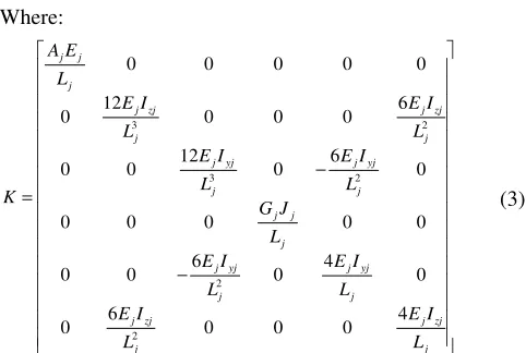
where λ is the proportionality coefficient between the force and displacement. This coefficient λ is function of the physical properties of the material, the relative position of point A, the application point of the load and the geometrical characteristics of the mechanical system. A straight bar j with a uniform cross section will soffer compliant displacement, when moments and forces acts on its extremities, as sketched in Fig. 1(a) and Fig. 1(b). Reference frames can be defined at the bar extremities i and i+1 where δx, δy, δz the linear compliant displacements while φx, φy, φz are the angular compliant displacements, along and about X-, Y- and Z- directions, respectively. Using the elastostatic properties of the bar one can obtain a 6x6 symmetrical stiffness matrix K that relates the applied forces/moments to compliant displacements in the form [4]:

= ∅ ∅ ∅ (2) Where:                                     − − = j zj j j zj j j yj j j yj j j j j j yj j j yj j j zj j j zj j j j j L I E L I E L I E L I E L J G L I E L I E L I E L I E L E A K 4 0 0 0 6 0 0 4 0 6 0 0 0 0 0 0 0 0 6 0 12 0 0 6 0 0 0 12 0 0 0 0 0 0 2 2 2 3 2 3 (3)

and Ej and Gj are the modulus of elasticity and the shear modulus of element j respectively; Lj is the beam length, Iyj, Izj are the moments of areas about the y and z axes, respectively, Jj is the Saint-Venant torsion constant and Aj is the cross-sectional area. The stiffness analysis enables to obtain the stiffness matrix K for a specific robotic structure at a given configuration. The compliance matrix C can be calculated as the inverse of the stiffness matrix K with deformations due to external loads. The main sources of robot structure compliance are the joints (including their actuators), and the links.

(a)

(b)

Figure 1 Forces and moments acting on a link (a); Compliant displacements due to forces and

Thus, according to the main compliance sources, several methods stiffness analysis have been proposed. One can organize the available methods into the following three groups [5]:

• Methods using lumped parameters; These methods can be divided into two main subgroups according to the used solving methods, namely those using the kinematic and dynamic forces distribution [9;15] and those using the Jacobian matrix [2;6-8;10-15].

• Methods using the Matrix Structural Analysis - MSA [5;16-20];

• Methods using the Finite Element Analysis – FEA [21;22].

It is noteworthy that each method has advantages and disadvantages and the choice of which to use will depend on the required accuracy of the results as well as the amount of computational time that can be considered as acceptable. Additionally, the choice of a specific formulation can also depend on the specific robotic architecture under investigation. In fact, some formulations require close-form kinematics equations that might be not straightforward as for example for some parallel robot architectures.

2.1 STIFFNESS MODEL USING LUMPED PARAMETERS

In general, Lumped parameter model (or lumped component model or lumped element model) is used to simplify the description of a physical system by using discrete entities that are equal or proportional to some average value of the corresponding distributed characteristics . The use of lumped parameters requires some assumptions. For the stiffness model for robotics in general the simplifying assumptions are that all links are rigid bodies with concentrated mass andthe interactions between rigid bodies take place via joints, springs and dampers and, the forces are concentrated. In the following two modeling methods are presented by using lumped parameters: namely, the method that uses the Jacobian matrix and the method that uses the kinematic and forces distribution.

2.1.1 Stiffness Models Using Jacobian Matrix

The Jacobian matrix methods have been studied by several authors as for example in [2;6-8;10-14].

These methods usually take into account only the joints as main compliance source. For a structure with n generalized coordinates and m operational coordinates the torque τ_{i, that}

is transmitted through the i-th joint can be related to the corresponding joint small deflections ∆qi by a linear approximation given as [2]:

= · (4)

where ki is called the joint stiffness constant (or lumped stiffness parameter). Equation (4) can be written in matrix form for the n generalized coordinates as

= · (5)

where τ _{= [}τ_1, τ_{2, ...,} τ_n]t_, ∆_q = [∆q1, ∆q2, ..., ∆qn]t and Kd= diag[k1, k2, ..., kn] a n x n diagonal matrix.

The vector of joint compliant displacements ∆_{qare related}

to the end-effector compliant displacements ∆_{x = [}δx δy δz φx φy φz], though the Jacobian matrix J given by:

= · (6)

The generalized forces F = [Fx Fy Fz Mx My Mz]t that are applied at the end-effector, , are related to joint reaction forces by the transposed Jacobian matrix of a robotic serial structure in the form:

= _{· (7)}

From Equations (4) to (7) one can obtain:

= · (8)

where = is the compliance matrix of the structure. When considering only the joint compliance the stiffness matrix Ks for serial robots can be obtained as:

! = = · · (9)

The compliant displacements due to links were addressed, for example by Komatsu et al. [10-12] in a study on serial robots. The flexibility for a serial structure, according to Yoon et al. [13-14] and Komatsu et al. [10-12] can be obtained using the Jacobian matrix by considering the structure composed of several deformable joints and deformable segments Cli where the joints flexibility are represented by Cjoint and the generalized coordinates are the angles θ_{i (i = 1,..., n).}

From those proposed method the segments and joints compliant displacements can be obtained as:

(

)

(

)

(

)

e T e e e T C C C diag C e J C e J C . . . , , 2 1 =

= θ θ

(10)

where CT is the compliance matrix of the end-effector, θ the angle of the joint, Je(θ,e) are the Jacobian matrices for each joint and each elastic deformation, Ce is the compliance matrix which is defined by the structural characteristics of all elements, Cej (j = 1, ... , n) is the compliance matrix of each element. For comparison purposes the effect of compliance links and joints can be considered separately by means of equations (4) to (8). In particular, the effect due to compliance links can be computed by means of the following relations:

"= "" "

"= #$%&( , ), … , +) (11) where Jl is the Jacobian Matrix that is obtained as function of ki (i = 1, ... , n) are the link lumped stiffness parameters. The amount due to joint compliance can be computed as:

-.= -. -. -.

-.= #$%&(- , -), … , -+) (12)

where Jart is the Jacobian Matrix of serial robotic structure and kai (i = 1,...,n) are the joint lumped stiffness parameters. Considering (11) and (12) one can rewrite (10) as:

/= "+ -. (13)

manipulators, where the point O is the origin (fixed platform) and a point P is the tip position of each limb (serial manipulator). Thus, the tip compliance matrix Cp, of parallel manipulator is given by:

1 1

2 1 1

1 − − −

−

+

+

+

=

p

C

C

C

C

L

where Csi (i = 1,…, n) is the compliance matrix of each serial manipulator obtained by Eq. (13). The mobile platform and fixed platform are considered as rigid bodies.

2.1.2 Formulation proposed by Tsai

The formulation proposed by Tsai in [2] can be considered equivalent to the model proposed by Komatsu et al. [10-12] when the links are rigid and taking into account only the compliance of joints. Thus, in this case, the calculation of compliance matrix for a serial robot structure can be obtained as:

=

= #$%&( , ), … , +) (15)

where J = Jart , K = Kart are given by (12) and ki=kai (i = 1, ..., n) are the joint lumped stiffness parameters. Tsai [2] assumes that, similar to serial manipulators, the links are perfectly rigid and he considers only the compliance of joints to obtain the stiffness matrix of a parallel manipulator.

In the case of parallel manipulators some joints are actuated and others are passive. Thus, it is not possible to obtain an independent function between the operational coordinates and generalized coordinates in the form:

1(, ) = 0 (16)

where f is a implicit function of the joint coordinates q and the end-effector coordinates x, and 0 is a zeroes vector. In this case, the joint compliant displacements ∆_{q are}

related with the end-effector compliant displacements ∆_x

given by:

– 4 = 0 (17)

where

= 51 (, )/5

4 = −51 (, ) / ∂ (18)

From (17) one can write

= 9∙ (19)

where 1

p q x

J =J J− is the Jacobian of a parallel manipulator. The relation between the torque and compliant displacements is given by:

= 9 (20)

The relation between the torque, τ_{, in the joints and the}

forces, F, at the mobile platform, is given by:

= 9 (21)

Substituting (20) int. (21) one can obtain:

= 9 9 (22)

or

= 9 (23)

where Kp =JpT Kd Jp is the stiffness matrix for parallel manipulators.

2.1.3 Model using the kinematic and dynamic forces distribution

This method is based on the computation and composition of 3 matrices as suggested in [9;15;23]. In this case the stiffness of a robot can be given by the stiffness of its components that are described by means of a suitable model of elastic response of those components. A suitable model can refer to lumped stiffness parameters for each component that can be identified by means of suitable linear and torsion springs and using the lumped stiffness model as in [9;15;23;25]. The stiffness matrix can be obtained numerically by defining an appropriate robot model, which takes into account the lumped stiffness model of the links and active joints. The method is also called as Component Matrix Formulation. The 3 matrices to be computed are A, B, D. The first matrix A gives the wrenches τ_{1 , … ,} τ_{n (n = numbers of components) acting on}

each component of the robotic system when a wrench τ _acts

on its end-effector in the form:

;= < ∙ (24)

with τ _L=(τ _{L1, … ,} τ _Ln)t_{. Therefore, matrix A is a 6n x 6}

matrix. The second matrix B gives the compliant displacements on the components when the wrenches τ _L

acts on the components and it can be expressed in the form:

== > ∙ ; (25)

where ∆_xL=(∆_{xL1 , … ,} ∆_xLn)t_{is a vector of the compliant}

displacements occurring to all the components of the architecture. Since ∆_{xL1 , … ,} ∆_{xLn are n vectors 6 x 1,} ∆_xL

is 6n x 1 and the matrix B is 6n x 6n matrix. If one writes

∆_xLi=Bi τ _{Li with (i=1,… , n) then the matrix B can be}

written as:             = n 1 B 0 0 0 0 ... 0 0 0 0 ... 0 0 0 0 B B (26)

The third matrix D is a 6 x 6n matrix that gives the compliant displacements occurring to the end-effector because of the compliant displacements on each component and it can be formulated in the form:

= ? ∙ = (27)

Equation (27) can be obtained by analyzing the kinematics of the manipulator and considering the variation of its kinematic variables due to the deformations and compliant displacements in the legs. Considering (24) to (27):

= (? > <) (28)

In this case this approach can be convenient for the computation of the stiffness matrix even for complex parallel or serial architectures as proposed in [9;23;24] for humanoid robots and parallel manipulators. However, special care has to be addressed in a proper choice of the subcomponents in order to getsquare invertible matrices. Thus, the stiffness matrix K can be computed as (28) that is a way to generalize the Jacobian formulation for clearly marking the dependencies with the 3 main aspects that influence the entries of the Cartesian stiffness matrix in equations (24) to (27).

2.2 STIFFNESS MODEL USING MSA

In this section the Matrix Structural Analysis (MSA) method, also known as the displacement method or direct stiffness method (DSM) is presented. Structural analysis methods break up a complex system into its component parts, making it a system of discrete structural elements with simple elastic and dynamic properties that can be readily expressed in a matrix form. Since a robotic system is made up of links and joints, this method makes it easy to determine the structure’s stiffness matrix. Discrete structures are composed of elements that are joined to each other by connecting nodes. When such a structure is loaded, each node suffers translations and/or rotations, which depend on the structure’s configuration and boundary conditions. The nodal displacement can be determined from a complete analysis of the structure. The matrices representing the links and joints are considered building blocks, which, when fitted together according to a set of rules derived from the theory of elasticity, provide the static and dynamic properties of the whole structure [16].

2.2.1. Stiffness of joints and links

The stiffness of a joint can be given by [19;20]:

@A+ = B ₋C_C −_CCD (29)

where Kc = diag(klx, kly, klz, kax, kay, kaz); klx, kly, klz are the coefficients for translational stiffness and kax, kay, kaz the coefficients for rotational stiffness about the x, y and z Cartesian axes. The stiffness matrix of a j-th three-dimensional straight bar (beam or link) with a uniform cross-sectional area can be expressed as:

@= B₋E@ −E@

E@ E@ D (30)

where Kbj is given by the matrix K from Eq. (3).

The application of MSA requires writing the stiffness matrices of all elements in the same reference frame before to assemble the stiffness matrix of the structure. The transformation matrix, Tjcan be obtained by linear algebra [4]. Thus, the stiffness matrix of the elements in a common reference frame (elementary stiffness matrix), for segments,

e j

k

k

@F= G@ @ G@ (31)

@A+F = G@ @A+ G@ (32)

After obtaining the stiffness matrix of links and joints in a common reference frame, the stiffness matrix of a structure can be determined using MSA. Based on how the structure elements are connected through their nodes, it is possible to define a connectivity matrix. Since segment and joint stiffness are known, the global stiffness matrix can be obtained by a superposition procedure described in [27]. The methodology described to obtain the global stiffness matrix considers the structure as free or, in other words, without motion constraints that make this matrix be singular. By applying boundary conditions when the displacements are known, a new invertible stiffness matrix K can be obtained, and the compliant displacement can then be computed as:

= (33)

where ∆_{x are the compliant displacements and F are the}

applied external wrenches. Methods based on matrix structural analysis are simple and easy to implement computationally. For example the authors of [25] used this approach to derive the stiffness matrix of each element of a Stewart platform and then their assemble the individual elements into the Stewart platform stiffness matrix. This approach is also used in [26] to obtain the stiffness model of a machine frame considered as a substructure. The superposition principle is used to obtain the stiffness model of the machine structure as a whole. Gonçalves [19] applied the MSA method for robotic systems and demonstrated the validity of this method by experimental tests in a structure composed by two links and one spherical joint simulating a closed kinematic chain. The errors between values obtained using MSA and experimental tests were small. Gonçalves and Carvalho [20] applied the MSA method in a 6-RSS parallel structure and once obtained errors compared with experimental results they considered acceptable the results in [27]. They applied the method to obtain the singularities of parallel robots too [18].

2.3 STIFFNESS MODEL USING FEA

Each element then is limited by points called nodes, and the group of elements with their nodes is called mesh. After the definition of elements and their respective nodes, inside each element one admits approximate solutions expressed by interpolation functions. It can be also imposed to conditions guarantee a continuous solution in the nodes shared by various elements. The problem’s unknowns, called dof, become the values of the field variables in the nodal points, and the number of these unknowns (now finite) is called number of degrees of freedom of the model. Depending on the nature of the problem, after the discretization, the governing mathematical model results on a finite number of ordinary differential equations or algebraic equations, where the numerical solution enables to evaluate the nodal unknowns. Once these unknowns are obtained, the values of the field variables inside the elements can be evaluated using interpolation functions [27]. Many authors have been using FEA for stiffness analysis of robotic structures. Bouzgarrou et al. [21] worked out a stiffness study of the parallel robot 3TR1 by using finite elements that are coupled to a CAD model. Clinton et al. [25] studied the stiffness of the Gough-Stewart platform with all elements subject only to traction and compression solicitations. Each element is studied individually and then assembled in order to study the structure as a whole. In Dong et al. [17] a study using FEA is elaborated in order to determine the stiffness model of a parallel structure that has flexure hinge joints. Zhou et al. [29] used FEA for the modeling of the parallel manipulator 3-PRS. The moving platform is modeled by triangular plate elements and the legs by beam spatial element. The flexibility of the joints is considered by the introduction of virtual springs to the FEA model. As the joints parameters are not known, the FEA numerical model is adjusted through experimental tests according to the frequency response functions. Deblaise [5;30] used FEA modeling to compare the results obtained using the MSA. This study was applied in the modeling of a Delta parallel robot. In the paper, a model considering only the flexibility of the segments not provided consistent results with experiments. Corradine et al. [22] used FEA to model the H4 robot. Besides the modeling of segments, the spherical and rotational joints were modeled introducing “displacement relaxation” in the FEA model, which allows, for the spherical joints, that all flexible translation displacements between the segments are the same, but not the rotations. For rotational joints all movements, excluding the rotation axis, should be the same. When comparing the results of the FEA model with those from experiments, they were close to each other. Kobel and Clavel [31] developed a reduced size with large workspace robot, named ΦR, for micro manipulation and assembling, using finite elements to evaluate the static behavior of the structure. The bearings in the structure were idealized using 6 springs between inner and outer rings of each revolute joint in order to account for the influence of such bearings. Aginaga et al. [32] presented an analytical method to calculate the stiffness matrix for parallel structures, applying it to the 6-RUS structure.

The finite elements method was then applied to a specific component of the structure, due to its complex geometry, in order to calculate the stiffness indexes of such component. Rezaei et al. [33] held the stiffness analysis of a spatial parallel 3-PSP structure considering the moving platform as flexible. The finite element method was then used as comparison parameter. Gonçalves and Carvalho [20] applied the FEA method to compare with results obtained by MSA method in a 6-RSS parallel structure. In general the FEA method is used to validate analytical models [5; 34-37] and or experimental results [5; 20-22; 29; 33] or even for optimization of structures and parts of structures [32; 38]. The biggest advantage of using the FEA method is the utilization of the mechanical design of structure’s project with no simplification, considering its full geometry. For robotic structures with irregular geometry, like industrial serial robots and parallel robotic structures that are subject to not only axial loads, like the Gough-Stewart platform, the use of the FEA method make the stiffness analysis for the robotic structure fairly easy . The disadvantage of the FEA method, when it involves commercial software for analysis, is that it requires great computational efforts, because, since stiffness depends on positions, it is necessary, for each specific position, to build a finite element model [26]. Other advantages of FEA are: elements of different shapes and sizes can be associated to discrete domains of complex geometry; the division of the continuous domain in regions makes the modeling of problems with non-homogeneous domains easier, where physical properties vary; and the method can completely formulated with matrices, making its computational implementation easier. The disadvantages of the method are the uncertainties inherent of the FEA modeling resultant of simplifications of the physical model such as: not considering some physical effects like non-linearity, hysteresis, damping; discretization error; inaccurate values of physical and/or geometrical parameters (elasticity models, density); difficulty in modeling localized effects such as screwed and errors derived of the process of numerical resolutions. A further key disadvantage is that a FEA meshing and calculation should be done for each single configuration of a robot structure.

3 CASES OF STUDY

In this section two cases of study are reported for the main techniques to obtain the compliant displacements. A first case of study refers to a 2 dof planar serial structure considering the compliance of links and joints. The second case of study deals with a prototype of a 6-RSS parallel structure. Finally experimental results are presented for stiffness evaluation. In both cases of study compliant displacements are used as local stiffness performance indices, as also proposed in [5].

Examples of calculation of the mechanical transmission mechanisms can be found in [1].

3.1 NUMERICAL SIMULATIONS APPLIED ON A SERIAL STRUCTURE

3.1.1 Methods based on Jacobian matrix

Figure 2 shows the sketch of a 2 dof planar serial robotic manipulator with the inertial reference frame O0 x0 y0, an reference frame Ax1 y1 fixed on the first link with length L1 and Bx2 y2 fixed on link with length L2. The angles θ1 and θ2 are the generalized coordinates (joints).

Figure 2 A 2 dof planar serial manipulator.

3.1.2 Applying the methods proposed by Yoon et al. [13-14] and Komatsu et al. [10-12]

Considering the compliant displacements for the scheme in Fig. 3, one can write the coordinates of points A and B as: HI= J cos(N) − sin (N)

QI= J sin(N ) + cos (N )

HR= HI+ J)cos(N + S + N)) − ) sin (N + S + N))

QR= QI+ J)sin(N + S + N)) − ) cos (N + S + N))

(34)

From Fig. 3(a) forces Fx and Fy applied at point B can be decomposed in the normal direction of links as, Fig. 3(b):

1 2 2

2

1 2

2

( ) cos( )

0

x y

y

y

F F sen F

F F

M L F

M θ θ = + = = = (35)

where F1 and F2 are the forces obtained from Fx and Fy applied at A and B, perpendicular to links 1 and 2, respectively. M1 and M2 are the moments applied at A and B, respectively, due to the force Fy. Applying the elastic differential linear equation [39] for a cantilever, the linear compliant displacements, δ1 and δ2, and angular compliant displacements φ1, φ2, due to the forces F1, F2, M1 and M2, are calculated by:

= 3VJTW + 2VJ)W )= J)

T

3V)W) )+

J))

2V)W) )

S = _2VJ)_W + _VJ_W S)= J)

)

2V)W) )+

J)

V)W) )

(36)

Substituting equation (35) into (36), and after mathematical manipulations, one can write the angular compliant displacement as [10-12]:

S = _2J3 + _2VW3V_(2J)W)J J)

) T_{+ 3J}

) )₎ )

S)= 3(J) )_{+ 2J}

))

2J)T+ 3J)) )

(37)

From Figures 6 and 7, the configuration of end-effector, point B, considering the kinematics model and compliant displacements is given by fT:

B B T x y θ     =      T f (38) where

N/= N + S + N)+ S) (39) The calculation of the links deformation is performed by Eq. (11) applied to the 2 dof serial manipulator:

"= "" "

"= #$%&( , )) (40)

As Jl is the Jacobian matrix it can be obtained by differentiating Eq. (38) related to deformations xl as:

H"= B

)D ; Jl ∂ = ∂ T l f x (41)

Then the Jacobian matrix can be obtained as:

11 12

21 22

31 32 l

Jl Jl

J Jl J

Jl Jl     =_{ }     (42) where

Z = −[$\(N) − T=]!+(^_)=b_`a)− Tc]CA!(^<sub>)=b</sub>_`a)

Z )= − Td]e]_f==b_]!+(^_dbeb_`a)− [$\(N-g) −Tc]d]e<sub>f=</sub>]=bCA!(^_`a)

]

]_dbeb

Z) = hi[(N) + T=]CA!(^_)=b_`a)− Tc]!+(^<sub>)=b</sub>_`a)

Z))= Td]e]_f==b_]CA!(^_dbeb_`a)+ hi[(N-g) −Tc]d]e<sub>f=</sub>]=b!+(^_`a)

]

]_dbeb

ZT = ₎₌T_b

ZT)= Td_f=]e]=b

]

]_dbeb+₎₌T_]

(43)

and

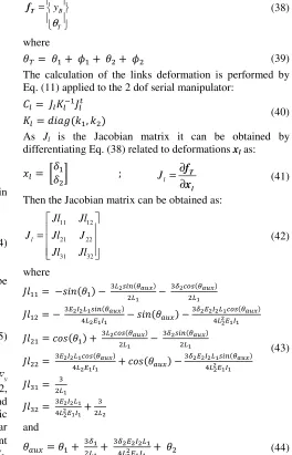
(a) (b)

Figure 3 Model for application of the methodology of Komatsu et al. [10-12] (a); Linear compliant displacement (δ1) and angular compliant displacement (φ1) (b).

Furthermore, to obtain the links compliant matrix, Eq. (40), it is necessary to determine the coefficients k1, k12 and k2, which are the lumped stiffness coefficients of the first link, the coupling between the links, and the second link, respectively. The calculation of these coefficients is accomplished by using the equation of strain energy for bending [39], Eq. (46), and the strain energy of the system related to δ1 and δ2, Eq. (45) [10-12]:

j = ( )+ )₂ )+ )))) (45)

(

)

(

)

0 2 2 2 2 2 2 1 0 2 1 1 1 1 1 2 1 2 1 2 1 dx M x F I E dx M x F I E U l l

∫

∫

Solving Equations (45) and (46), and after mathematical simplifications, it can be obtained as:

3 1 1 1 1 3 L I E

k = ₍₄₇₎

0

=

k

k = − θ + + (49)

Thus, one can obtain Cl by replacing Eqs. (47) to (49) and (36) into Eq. (42).

The calculation of the compliance matrix due to joints is obtained by applying Eq. (12) to the model of Fig. 6.

)

,

(

1 a a art T art art art art

k

k

diag

k

J

k

J

C

=

=

The calculation of the Jacobian matrix due to joints, Jart, is given by differentiating Eq. (38) related to xart as:

art

J

=

∂

∂

f

x

where θ_{aux is given by Eq. (44). The values of the stiffness}

constants ka1 and ka2 can be done by experimental data or from catalogs. Thus, it is possible, from Eqs. (51) and (52), to obtain the compliance matrix due to the joints.

-.= k

−J [$\(N ) − hi[(N ) − J)[$\(N-g) − )hi[(N-g) − J)[$\(N-g) − )hi[(N-g)

J hi[(N) − [$\(N ) + J)hi[(N-g) − )[$\(N-g) J)hi[(N-g) − )[$\(N-g)

1 1 m

Finally, the compliance matrix of the 2 dof serial robotic manipulator is given by:

CT = Cl + Cart (53)

The stiffness matrix can be calculated as the inverse of CT.

3.1.3 Matrix Structural Analysis – MSA method

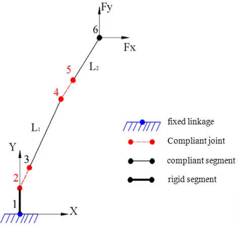
In this section, the stiffness matrix is obtained using the Matrix Structural Analysis (MSA). Figure 4 illustrates a model for application of the MSA methodology.

Figure 4 Nodes in the 2 dof serial manipulator for applying the MSA method.

In Figure 4, points 1 to 6 are the nodes, the segment defined by the nodes 1-2 is considered a rigid base and the links defined by the nodes 3-4 and 5-6 are flexible.

The rotational joints are represented by nodes 2-3 and 4-5. It should be emphasized that the nodes which define the rotational joint have the same position. The inertial frame has its origin at node 1. Firstly the stiffness matrices of each element are obtained both for the three segments and two joints. To obtain the stiffness matrix relative to the segments, they are considered as beam elements with circular cross section, neglecting the effects of shear forces that are calculated by Eq. (3). The joint stiffness matrix is given by Eq. (29). In order to obtain the joint compliance matrix the linear stiffness parameters klx, kly, klz and angular stiffness parameters kax, kay, kaz can be obtained according to the manufacturers' catalog or by experimental tests. Before performing the assembly of the stiffness matrix of the manipulator as a whole the matrices of each element relative to the inertial frame Oxyz must be written using the transformation matrix Tj, Eqs. (31) and (32). The nodes coordinates 1 to 6 are obtained by the kinematics model of the robot. The segment defined by nodes 1 and 2, corresponding to the base of the robot, can be considered flexible or not. In this example it is considered as rigid segment. For this, in this element stiffness matrix is considered its modulus of elasticity as 10 times larger than the other segments. From the segments and joints stiffness matrix in relation to the inertial frame can be done the assembly of the stiffness matrix of the whole structure. Since each node has 6 dof, the size of this square matrix is 6n = 36. The assembly of this matrix must conform to the numbering of the nodes shown in Fig. 4. Thus it is possible to establish a connectivity matrix between elements, which indicates, for example, nodes 2 and 3 (forming a rotational joint) have the same linear displacement and angular displacement, except the rotation around the joint axis. Thus, Fig. 4 and Table I, for each node is reported the quantification of dof which represents the number of possible movements.

Table I - Degrees of freedom related to Fig. 4

Nodes

Compliant Displacement 1 2 3 4 5 6

Linear compliant displacement on x direction (δx) 1 7 13 19 25 31 Linear compliant displacement on y direction (δy) 2 8 14 20 26 32 Linear compliant displacement on z direction (δz) 3 9 15 21 27 33 Angular compliant displacement around x (φx) 4 10 16 22 28 34 Angular compliant displacement around y (φy) 5 11 17 23 29 35 Angular compliant displacement aroundz (φz) 6 12 18 24 30 36

The connectivity matrix can be written as

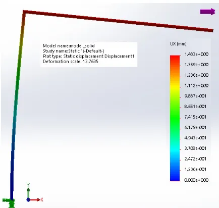
Figure 5 FEA model compliant displacements.

The connectivity matrix allows the stiffness matrix assembly of the whole structure. This provides the element position inside the structure stiffness matrix. The obtained matrix is singular because the structure has no restrictions. So, must be applied the boundary condition that, in this case corresponds to a fixed node 1. As in the fixed node all displacements are zero one can eliminate these degrees of freedom of the system (1-6), corresponding to node 1.Thus, the new square matrix is a 30x30 dimensional and is invertible. This procedure is detailed in [27]. In Fig. 4 forces can be applied in all nodes. In this example forces are applied only at node 6, for comparison with other methodologies. Thus, the compliant displacements can be calculated by Eq. (33),where K is a 30x30 matrix and the vector F, applied in the nodes 2-6 is a 30x1 vector and the flexible displacement vector ∆_{x is a 30x1 vector.}

3.1.4 FEA Model -Finite Element Analysis

The example for finite element model and simulation has been carried out by using the commercial software SolidWorks®. The proposed model takes into account only the compliance of links that have modeled as solid body.. Figure 5 presents the model of a 2 dof robotic manipulator at a specific configuration (θ1 = 90º and θ2 = -90º). Elements discretization has been defined by software default. The compliant displacements have been calculated by applying a unit force along x axis.

3.1.5 Comparison and discussion between the results of serial structure

Tables II, III and IV summarize a comparison the methodologies presented by Komatsu et al. and Yoon et al., Tsai, MSA and FEA referring to displacements at point B of 2 dof robotic manipulator configuration that is shown in Fig.3, with: θ1 = 90º and θ2 = -90º. Unit force have been applied along the x axis, (Fx = 1 N and Fy = 0). For all models, the links have been considered as made of steel with elastic modulus E = 2e11N/m2 with a length of 0.3 m and circular cross section with a diameter of 0.005 m.

The joints lumped parameters for the models of Komatsu et al., Yoon et al. and Tsai have been set as equal to:

ka1 = ka2 = 1000 N m/rad (55) For the joint compliance simulation using the MSA the following values have been considered for numerical simulation:

klx = kly = klz = 2e11 N/m kax = kay = 2e11 N m/rad kaz = 1000 N m/rad

(56)

It has been also assumed kaz = ka1 = ka2.

Table II presents a comparison of results when using only the joints compliance, and segments are rigid. Table III shows the results when considering only the segments flexibility and neglecting the joints flexibility. Table IV presents the results considering both the flexibility of joints and segments.

When considering only the joints flexibility as in Table II, the results using the method of Komatsu et al. and Yoon et al. provide the same results when compared with the model used by Tsai. This is expected because both methods use the calculation of Jacobian matrix. In the procudere using the MSA results are different due to the no knowledge of values corresponding to klx, kly, klz, kax and kay. A more close match with the data used by Komatsu et al. and Yoon et al. could be achieved by more accurate matching of the above parameters in the two different models. Considering the model with only the segments flexibility as in Table III, the results are coincident in the methods MSA and FEA and with the methodology of Komatsu et al. and Yoon et al. results are quite similar. By considering joints and segments flexibilities as inTable IV, the results from the procedures of Komatsu et al. and Yoon et al. and MSA are close. Considering only the flexibility of joints as in Table II, the model proposed by Tsai is more convenient since it is derived from the calculation of the Jacobian of the robotic structure. But the calculation of this Jacobian can become complicated when depending on the number of structured and type of structure considered. For example, for a parallel robotic structure the Jacobian matrix is not simple.

When considering only the segments flexibility as in Table III, using the MSA method is more favorable because unlike the methodology used by Komatsu et al. and Yoon et al., it is not necessary to calculate differential equations, it is the case for calculating the Jacobian considering the segments flexibility. As shown by Eqs. (34) to (54) this calculation can be complicated and susceptible to errors. In this example a 2 dof serial robotic manipulator is considered. If the number of dofs is larger, more calculations of differential equations are necessary. Furthermore, the methodology of Komatsu et al. and Yoon et al. requires to calculate the value of the forces acting on each segment, and the computation can be complicated depending on the number of segments and forces and/or moments in the model.

Table II - Results of compliant displacements considering only the joints flexibility

Compliant Displacements

Methodologies Komatsu et al. and

Yoon et al. Tsai MSA Computational time [s] 0.21 0.01 0.183

δx [mm] 0.09 0.09 0.2518

δy [mm] -0.09 -0.09 -0.3249

δz [mm] 0 0 0

φx [rad] 0 0 0

φy [rad] 0 0 0

φz [rad] 0 0 -0.0011

Table III - Results of compliant displacements considering only the segments flexibility

Compliant Displacements

Methodologies Komatsu et al. and

Yoon et al. MSA FEA Computational time [s] 3.095 0.109 3.0

δx [mm] 1.4347 1.4668 1.483

δy [mm] -2.1676 -2.2001 -2.198

δz [mm] 0 0 0

φx [rad] 0 0 0

φy [rad] 0 0 0

φz [rad] -0.0073 -0.0073 0

Table IV - Results of compliant displacements considering the joints and segments flexibilities

Compliant Displacements

Methodologies Komatsu et al. and

Yoon et al. MSA Computational time [s] 3.49 0.1818

δx [mm] 1.5234 1.5720

δy [mm] -2.2567 -2.3050

δz [mm] 0 0

φx [rad] 0 0

φy [rad] 0 0

φz [rad] -0.0073 -0.0076

3.2 NUMERICAL AND EXPERIMENTAL RESULTS FOR PARALLEL ROBOTS

3.2.1 A 6-RSS parallel structure

The 6-RSS parallel structure is a 6 dof manipulator, which is characterized by a base and a mobile platform, connected by six RS-SS segments, where the R-joint is on the reference frames, two joints by axis. The S-joints on the other extremity of the links are connected at the mobile platform, consisting in a virtual cube where the S-joints are tied on the center of its faces three crossed segments. Kinematics variables are the input angles αi (i=1 to 6) of the R-joints. The studied structure has the RS-segment and the SS-segment with the same length i.e., |b1b2 | = |b3b4 | = |

b5b6 | = | p1p2 | = | p3p4 | = | p5p6 |, Fig. 6(a). Figure 6(b) show

a prototype built at the Laboratory of Automation and Robotics in Uberlandia,Brazil.Kinematic analysis can be obtained by using a suitable analytical procedure with a vector and matrix formulation as reported in [27].

(a)

(b)

Figure 6 (a) The 6-RSS parallel structure with generic configuration; (b) The built prototype.

Figure 7 A Stiffness Model for the 6-RSS Parallel Manipulator with lumped stiffness parameters.

3.2.3 Structural Analysis with MSA and FEA methods. In this section the stiffness model of the 6-RSS parallel structure is presented considering the compliance of links and joints. The arms and forearms are modeled as beams and the stiffness analysis of the structure is carried out according to the elements that are considered in the structure as in Fig. 8. The following parameters were used in the model: length of the arms and forearms equal to 0.3m; |b1b2 | = |b3b4 | = | b5b6 | = | p1p2 | = | p3p4 | = | p5p6 | = 0.076m; the segments are built of steel with (E = 2 x 1011 N/m2 and G = 0.8 x 1011 N/m2) the cross-sectional is circular with 0.005m diameter.

The boundary conditions are given by actuators, that are considered as blocked and, therefore, the forearms can be considered as fixed in the rotational joints (nodes 1, 7, 8, 13, 14 and 19). The external force and torque are applied on node 4, which is the center of the mobile platform. Numerical simulations had been carried out considering both stiffness for links and joints, using translational and rotational stiffness for joints with values in (57) given by: klx = kly = klz = 2e11 N/m; kax = kay = kaz =0 Nm/rad (57) From the nodes that are defined on Fig. 8(b), the structure has 19 nodes with 6 dofs in each node. Thus, the system has 114 dofs with a 18x12 connectivity matrix. The stiffness matrix of the structure after considering the boundary conditions (six fixed rotational joints) becomes a 78x78 matrix. In order to verify the presented analysis using the MSA method, a model was built in FEA using commercial Ansys® software. The used element is a beam type divided in 10 parts. This model does not consider the joint stiffness. Table V provides results that are obtained from the FEA and MSA models. In Table 5 Fe is the external force Fe = [Fx, Fy, Fz] and Me the external torque Me = [Mx, My, Mz]. Results of numerical simulations are presented in Table 5. The results show the soundness of the model also in terms of symmetry of the structure.

One can note that the compliant displacements are the same in the direction of the applied forces when other forces and torques are zero and, if the same effort values are applied, the compliant displacements are equals.

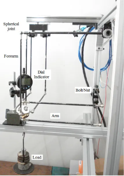
A non-actuated prototype of the 6-RSS was built for experimental tests, Fig. 9. The actuators, which are blocked with bolts and nuts, are used as boundary conditions (nodes 1, 7, 8, 13, 14 and 19), so that the rotational joints can be considered as fixed. Tests were performed with the measurement of compliant displacements in one direction, using a dial indicator. Three different loads P1 = 0.9935 kg, P2 = 1.2435 kg and P3 = 1.4915 kg were applied on the center of the platform, at node 4. The acceleration of gravity is g = 9.81 m/s2. These experimental tests were performed with an initial 6-RSS Parallel Manipulator configuration of α1 = α2 = α3 = α4 = α5 = α6 = 0°.

(a) (b)

Figure 8 A Stiffness model of a 6-RSS parallel architecture: (a) 3D sketch; (b) Nodal points at joints.

Figure 9 Layout for Experimental stiffness tests of 6-RSS using a dial indicator.

Table V - Computed displacements of node 4 for α1=α2=α3=α4=α5=α6= 0° (Forces are given in [N] and torques in [Nm]) U δx[m] δy[m] δz[m] φx[rad] φy[rad] φz[rad]

Fe=(10,0,0) Me=(0,0,0)

MSA 0.002168 -0.000532 -0.000532 0.000857 0.001701 -0.005384 FEA 0.002173 -0.000534 -0.000534 0.000854 0.001727 -0.005378 Fe=(0,10,0)

Me=(0,0,0)

MSA -0.000532 0.002168 -0.000532 -0.005384 0.000857 0.001701 FEA -0.000534 0.002173 -0.000534 -0.005378 0.000854 0.001727 Fe=(0,0,10)

Me=(0,0,0)

MSA -0.000532 -0.000532 0.002168 0.001701 -0.005384 0.000857 FEA -0.000534 -0.000534 0.002173 0.001727 -0.005378 0.000854 Fe=(10,10,10)

Me=(0,0,0)

The results shown in Table VI confirm the validity of the MSA method by which the compliant displacements in the direction of applied force were obtained with an error of less than 9%. Although the FEA and MSA methods use the same equations (29) to (33), the MSA method offers several advantages such as: (a) A robotic structure is composed by links and joints that can be modeled by only two nodes in the MSA method. In contrast, the FEA method needs to divide each link into several nodes. (b) Commercial FEA software do not allow for control of the solver. In contrast, the MSA method allows the assembly of the stiffness matrix to be followed step-by-step. (c) In the FEA method, each change in the structure’s configuration requires to redo the mesh, thus increasing the computational cost.

The MSA method requires only an improvement of the inverse kinematic model to map the stiffness of all the configurations of the structure.

Table VI - Measured Compliant displacements of nodes with test-bed in Fig. 3.

Load

δy

MSA [mm]

Average experimental

[mm]

Standard deviation

[mm]

Error [%]

Node 17

P1 2.136 1.995 0.047 6.6 P2 2.673 2.696 0.047 0.9 P3 3.206 3.201 0.049 0.16

Node 11

P1 2.250 2.058 0.030 8.5 P2 2.817 2.736 0.028 2.9 P3 3.378 3.460 0.004 2.4

Node 5

P1 2.062 1.897 0.015 8 P2 2.581 2.540 0.010 1.7 P3 3.096 3.260 0.012 5.3

Node 3

P1 2.062 2.013 0.004 2.4 P2 2.581 2.731 0.009 5.8 P3 3.438 3.663 0.030 6.5

4 CONCLUSIONS

This paper provides a comparison among the main methods for calculating the compliant displacements in robotic structures. In particular, the main available methodologies and formulations have been described and applied to two specific cases of study, namely, a 2 dof serial robotic manipulator and a 6 dof parallel manipulator. The results were compared also through experimental tests.

The experimental results confirm the validity of the MSA and FEA models, that can obtain an accurate estimation of compliant displacements along the direction of applied force.

MSA method is found to require less computational efforts as compared with FEA also because FEA requires a re-modeling and re-meshing at any robot configuration. Lumped stiffness parameters methods can have lower accuracy, but, they can provide a much quicker analysis of the stiffness performance over the whole robot workspace. It is to note that some lumped parameter and Jacobian methods can require complex preliminary calculations of the kinematics/statics models. Accordingly, these methods should not be used when proper close form equations are not available. Additionally, for the choice of a specific stiffness analysis formulation it plays a key role to identify the desired level of accuracy as well as the components that are seen as minimally contributing to the structure compliance so that they can be considered as negligible.

5 ACKNOWLEDGEMENTS

The authors are thankful to CNPq, CAPES and FAPEMIG for the partial financing support of this research work.

REFERENCES

[1] E.I. Rivin. Stiffness and Damping in Mechanical Design. Marcel Dekker Inc., New York,1999.

[2] L.W. Tsai. Robot Analysis: The Mechanics of Serial and Parallel Manipulators. John Wiley & Sons, New York, 1999.

[3] W.K. Yoon, T. Suehiro, Y. Tsumaki and M. Uchiyama. Stiffness Analysis and Design of a Compact Modified Delta Parallel Mechanism. Robotica, Vol. 22, pp.463-475, 2004.

[4] A.A. Shabana. Dynamics of Multibody Systems. John Wiley & Sons, 1989.

[5] D. Deblaise, X. Hernot and P. Maurine. A Systematic Analytical Method for PKM Stiffness Matrix Calculation. Proc. of IEEE Int. Conf. on Robotics and Automation - ICRA 2006, 2006.

[6] D. Zhang, F. Xi, C.M. Mechefske and S.Y.T. Lang. Analysis of Parallel Kinematic Machine with Kinetostatic Modeling Method. Robotics and Computer-Integrated Manufacturing, Vol. 20, No. 02, pp.151-165, 2004.

[7] F. Majou, C.M. Gosselin, P. Wenger and D. Chablat. Parametric Stiffness Analysis of the Orthoglide. Proc. of the 35th Int. Symp. on Robotics, Paris, 2004. [8] O. Company, F. Pierrot and J.C. Fauroux. A Method

for Modeling Analytical Stiffness of a Lower Mobility Parallel Manipulator. Proc. of IEEE ICRA: Int. Conf. on Robotic and Automation, Barcelona, Spain, 2005. [9] M. Ceccarelli and G. Carbone. A Stiffness Analysis

for CaPaMan (Cassino Parallel Manipulator). Mechanism and Machine Theory, Vol. 37, pp.427-439, 2002.

[11] T. Komatsu, M. Uenohara, S. Iikura, H. Miura and I. Shimoyama. Dynamic Control for Two-Link Flexible Manipulator. The Japan Society of Mechanical Engineers (in Japanese), 1989.

[12] T. Komatsu, M. Uenohara, S. Iikura, H. Miura and I. Shimoyama. Vibration Control for Two-Link Flexible Manipulator using a Wrist Force Sensor. The Japan Society of Mechanical Engineers (in Japanese), 1990. [13] W.K. Yoon, T. Suehiro, Y. Tsumaki and M.

Uchiyama. Stiffness Analysis and Design of a Compact Modified Delta Parallel Mechanism. Robotica, Vol. 22, pp. 463-475, 2004.

[14] W.K. Yoon, T. Suehiro, Y. Tsumaki and M. Uchiyama. A Method for Analyzing Parallel Mechanism Stiffness Including Elastic Deformations in the Structure. Proc. of the IEEE/RSJ Int. Conf. on Intelligent Robots and Systems IROS’02, Lausanne, pp. 2875-2880, 2002.

[15] M. Ceccarelli, Fundamentals of Mechanics of Robotic Manipulation, Kluwer, Dordrecht, 2004.

[16] J.S. Przemieniecki. Theory of Matrix Structural Analysis. Dover Publications, Inc, New York, 1985. [17] W. Dong, Z. Du and L. Sun. Stiffness Influence

Atlases of a Novel Flexure Hinge-Based Parallel Mechanism with Large Workspace. Proc. of IEEE ICRA: Int. Conf. on Robotic and Automation, Barcelona, Spain, 2005.

[18] R.S. Gonçalves and J.C.M. Carvalho. Singularities of Parallel Robots Using Matrix Structural Analysis. Proc. of the XIII Int. Symp. on Dynamic Problems of Mechanics, Angra dos Reis, RJ, Brazil, 2009.

[19] R.S. Gonçalves, Estudo de Rigidez de Cadeias Cinemáticas Fechadas (Stiffness Analysis of Closed Loop Kinematic Chains). Universidade Federal de Uberlândia. Thesis (in Portuguese), 2009.

[20] R.S. Gonçalves and J.C.M. Carvalho. Stiffness Analysis of Parallel Manipulator Using Matrix Structural Analysis. EUCOMES 2008, 2nd European Conf. on Mechanism Science, Cassino, Italy, 2008. [21] B.C. Bouzgarrou, J.C. Fauroux, G. Gogua and Y.

Heerah. Rigidity Analysis of T3R1 Parallel Robot with Uncoupled Kinematic. Proc. of the 35th Int. Symp. on Robotics, Paris, France, 2004.

[22] C. Corradini, J.C. Fauroux, S. Krut and O. Company. Evaluation of a 4 Degree of Freedom Parallel Manipulator Stiffness. Proc. of the 11th Word Cong. In Mechanism & Machine Science, IFTOMM 2004, Tianjin, China, 2004.

[23] M. Ceccarelli. A Stiffness Analysis for CaPaMan. Proc. of Conf. on New Machine Concepts for Handing Manufacturing Device on the Basis of Parallel Structures, VDI 1427, Braunschweig, pp. 67-80, 1998. [24] G. Carbone, H.O. Lim, A. Takanishi and M.

Ceccarelli. Stiffness Analysis of the Humanoid Robot WABIAN-RIV: Modelling. IEEE Int. Conf. on Robotics and Automation ICRA 2003, Taipei, paper ID10615, 2003.

[25] C.M. Clinton, G. Zhang, and A.L. Wavering. Stiffness Modeling of a Stewart-Platform-Based Milling Machine. In Trans. of the North America Manufacturing Research Institution of SME, Vol. 25, pp. 335-340, Lincoln, 1997.

[26] T. Huang, X. Zhao, and D.J. Whitehouse. Stiffness Estimation of a Tripod-Based Parallel Kinematic Machine, IEEE Trans. on Robotics and Automation, Vol. 18, No. 1, 2002.

[27] G.D.L. Soares Jr, J.C.M. Carvalho and R.S. Gonçalves, Stiffness Analysis of multibody systems using matrix structural analysis MSA. Robotica, pp. 1-18, 2015

[28] S.C. Brenner and L.R. Scott. The Mathematical Theory of Finite Element Methods, Texts in Applied Mathematics, Vol. 15, Springer, 2008.

[29] Z. Zhou, J. Xi and C.K. Mechefske. Modeling of a Fully Flexible 3PRS Manipulator for Vibration Analysis, Journal of Mechanical Design, Vol. 128, pp. 403-412, 2006.

[30] D. Deblaise. Contribution à la Modélisation et à L’étalonnage Elasto-Géométriques des Manipulateurs à Structure Parallèle, Thesis, INSA Rennes, 2006. [31] P. Kobel and R. Clavel. Micro Robot for Rotary

Desktop Assembly Line. Proc. of IEEE International Symposium on Assembly and Manufacturing, 2011. [32] J. Aginaga, I. Zabalza, O. Altuzarra and J. Nájera.

Improving Static Stiffness of the 6-RUS Parallel Manipulator Using Inverse Singularities. Robotics and Computer-Integrated Manufacturing 28, Spain, 2012. [33] A. Rezaei, A. Akbarzadeh and M. Akbarzadeh. An

Investigation on Stiffness of a 3-PSP Spatial Parallel Mechanism with Flexible Moving Platform Using Invariant Form. Mechanism and Machine Theory 51, 2012.

[34] B.S. El-Khasawneh and P.M. Ferreira. Computation of Stiffness and Stiffness Bounds for Parallel Link Manipulator. Int. J. Machine Tools & Manufacture, Vol. 39, No. 02, pp. 321-342, 1999.

[35] Y.W. Li, J.S. Wang and L.P. Wang. Stiffness Analysis of a Stewart Platform-Based Parallel Kinematic Machine, Proc. of IEEE ICRA: Int. Conf. on Robotics and Automation, Washington, US, 2002.

[36] Q. Liang, D. Zhang, Z. Chi, Q. Song and Y. Ge. Six-dof Micro-Manipulator Based on Compliant Parallel Mechanism with Integrated Force Sensor. Robotics and Computer-Integrated Manufacturing 27, China, 2011.

[37] A. Taghvaeipour, J. Angeles and L. Lessard. Online Computation of the Stiffness Matrix in Robotic Structures Using Finite Element Analysis. Department of Mechanical Engineering and Centre for Intelligent Machines, McGill University, Canada, 2010.

[39] F.P. Beer, E.R. Johnston, J.T. De Wolf and D.F. Mazurek. Mechanics of Material, 5th Ed., United States, 2009.

[40] G. Carbone, Stiffness Analysis and Experimental Validation of Robotic Systems, Frontiers of Mechanical Engineering, Vol. 06, No. 02, pp. 182-196, 2011.

57

TEMPLATE FOR PREPARING PAPERS FOR PUBLISHING IN

INTERNATIONAL JOURNAL OF MECHANICS AND CONTROL

Author1* Author2**