of the core material used. It is important that the parameters extracted for the hysteresis model be optimized across the range of operating conditions that may occur in circuit simulation. This paper shows how to extract optimal parameters for the Jiles–Atherton model of hysteresis by the genetic algorithm ap-proach. It compares performance with the well-known simulated annealing method and demonstrates that improved results may be obtained with the genetic algorithm. It also shows that a combination of the genetic algorithm and the simulated annealing method can provide an even more accurate solution than either method on its own. A statistical analysis shows that the optimiza-tion obtained by the genetic algorithm is better on average, not just on a one-off test basis. The paper introduces and applies the concept of simultaneous optimization for major and minor hysteresis loops to ensure accurate model optimization over a wide variety of operating conditions. It proposes a modification to the Jiles–Atherton model to allow improved accuracy in the modeling of the major loop.
Index Terms—Circuit simulation, genetic algorithm, hysteresis,
Jiles–Atherton, magnetic component modeling, optimization.
I. INTRODUCTION
T
RANSFORMERS and inductors are essential components in a wide variety of power and communications applica-tions, and the accurate modeling of these devices for use in cir-cuit simulation is essential to predict design performance. It is required to accurately represent the hysteresis behavior of the magnetic core material used in these components in the sim-ulation model. One model that has been used quite widely is that of Jiles and Atherton [1], [2]. Jiles et al. [7] show how the parameters for the model may be extracted from a set of mea-sured data for a major hysteresis loop but do not consider arbi-trary loop sizes, and Prozygy [8] has established the effects of parameter variations on the major loop. Optimization methods applied to fit the Jiles–Atherton hysteresis loops to measured data have been investigated by Schmidt and Guldner [9], and Lederer et al. [10] using the well-known simulated annealing approach. Genetic algorithms provide an alternative approach to optimization which may have some advantages, especially when considering the more complex problem of fitting several loops simultaneously.Manuscript received June 16, 2000. This work was supported in part by the Engineering and Physical Sciences Research Council and Advanced Power Components Ltd., both in the U.K.
The authors are with the Department of Electronics and Computer Sci-ence, University of Southampton, Highfield, Southampton, U.K. (e-mail: [email protected]; [email protected]; [email protected]).
Publisher Item Identifier S 0018-9464(01)01822-2.
difficult engineering problems is a relatively recent innova-tion. Holland [3] and Goldberg [4] are two of the pioneers of this technique, and the last 10 yr have seen a plethora of applications for genetic algorithms from systems design to topology analysis [5]. The fundamental difference between genetic algorithms and conventional optimization techniques, such as simulated annealing [6], is that in certain problems, the computational effort involved in a standard exhaustive search method would be prohibitive. The random nature of genetic algorithms may not find the absolute best solution, but it has a greater chance of finding a good solution, quickly, for difficult problems. This randomness also works well for problems with chaotic or ill-defined behavior difficult to classify, and those problems with local maxima or minima that would perhaps trap a conventional search algorithm.
The optimization of magnetic materials is a problem which has aspects suited to the application of genetic algorithms. Even though the Jiles–Atherton [1] model of hysteresis is well under-stood mathematically, the parameters are interlinked in such a way that the set of possible combinations of parameters may be large. Significant changes in the shape of the hysteresis loop may result from small parameter variations. These two aspects give a relatively high risk of local maxima or minima being found or instabilities in a conventional algorithm. Other ap-proaches for modeling magnetic materials such as the Preisach [11] model have no direct link between behavior and material physical properties so are natural potential targets for the ge-netic algorithm approach.
II. OUTLINE OF THEGENETICALGORITHMMETHOD
A. Overview
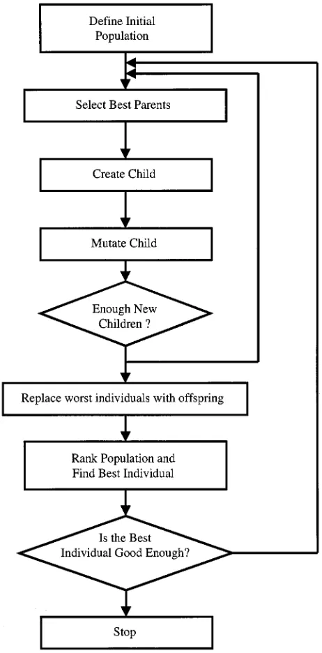
The flowchart of a generic genetic algorithm is shown in Fig. 1. The algorithm is based on the concept of natural selec-tion. The first step is to define an initial population of individ-uals, or set of magnetic model parameters, which is the first gen-eration for the algorithm. In this application, the initial popula-tion is formed by taking an initial set of parameters which are then subjected to random variations.
B. Choosing Parents
For each generation, there will be a number of children cre-ated by combining the characteristics of two parent individuals. The choice of parents is determined by random and selective methods. First, a set of possible parents is randomly chosen from the current generation. The prospective parents are then ranked
Fig. 1. Generic genetic algorithm method.
in terms of a fitness function to find the best individual, which is then chosen as the first parent. In this case, the fitness function is a measure of how closely the BH (flux density-B versus mag-netic field strength-H) curve matches the target. This process is repeated with a new set of possible parents to find the second parent. Once the two parents have been selected, then their char-acteristics can be combined to create a new individual (child).
C. Creating New Children
[image:2.612.50.281.69.537.2]A new child is created by the random combination of the characteristics of the parents. The overall set of parameters is defined as a string (chromosome) made up of individual param-eters (genes). Each parameter is represented by a floating-point binary number. The child’s chromosome is then constructed by
Fig. 2. Genetic algorithm crossover.
combining the genes of the parents using a crossover method, il-lustrated in Fig. 2. The selection of parents and creation of new individuals (children) is then repeated until the specified number of children is achieved.
As in natural reproduction, there is a risk of mutation during the crossover process. This is implemented by adding random changes to a proportion of the children created.
D. Renewing the Population
Once the required number of children has been created, the population as a whole is adjusted, in this case keeping the size of the population constant. To do this, the parent’s generation is tested for fitness, ranked, and the worst individuals replaced by the children.
The new generation is again ranked using the fitness function, and the best individual is evaluated to see if it meets the require-ments of the goal function, and if so, the algorithm stops; oth-erwise, the algorithm can continue.
III. FITNESS ORGOALFUNCTIONS
The fitness, or goal, function that defines the performance of the model is based on a simple least squares error approach comparing the curve(s) with the target on a point-by-point basis. An alternative goal function described by Wilson and Ross [12] has been implemented based on performance metrics such as initial permeability, saturation flux, and energy loss. By using weighting of metrics, the goal function is made appropriate for the ultimate application.
IV. OPTIMIZING THEJILES–ATHERTONMODEL OFHYSTERESIS
A. Jiles–Atherton Model
The Jiles and Atherton [1], [2] model of hysteresis is a phys-ically based approach for modeling magnetic hysteresis. The parameters of the model are related to physical features in the model such as the saturation magnetization, summarized as fol-lows:
irreversible loss; anhysteretic behavior;
reversible/irreversible proportions; effective field;
the loss can be made a function of the applied field or the flux density and propose a linear function. It was found, however, that a Gaussian function of the form shown in (1) gave excellent results, and this was therefore used in this paper. This function has the added advantage of no discontinuity around zero when the applied field changes polarity which improves simulation convergence.
(1)
where
default value of the parameter; applied field;
standard deviation of the Gaussian function.
Tests with materials such as 3F3 and N30 have demonstrated a significant improvement in the accuracy of the modeled curves.
C. Applying the Genetic Algorithm Approach
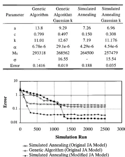
A toroid made of the Siemens N30 material was tested, and the resulting BH loop used for optimization. The Jiles–Atherton model was optimized using the classical model and also the im-proved model utilizing the variable parameter. The optimiza-tion was carried out using the well-understood simulated an-nealing method as a control and also with a genetic algorithm approach. The simulated annealing approach was carried out with a variation of 10%, a control factor of 0.001, and 2500 it-erations used. The genetic algorithm used 50 genit-erations of a population including 50 individuals (50 times 50 giving a rough equivalent of 2500 iterations). Each generation produced 40 children of whom 20 were mutated. A variation of 10% was in-troduced in the mutation process. In each case, the fitness func-tion used the least squares error approach.
The resulting mean errors between the simulated and mea-sured results are summarized in Table I and Fig. 3. Table I shows the error is significantly reduced for the genetic algorithm and that the variable parameter makes a significant difference for both optimization methods. Fig. 3 shows the error versus the number of iterations and again clearly, the genetic algorithm with the Gaussian modification of is the best result.
[image:3.612.300.554.92.411.2]Interestingly, when a combination of simulated annealing and the genetic algorithm was applied, an even better result was achieved. This can be explained with the fact that the two methods have different strengths. The genetic algorithm is very good at finding the correct area of the solution, tolerant of local maxima and minima, and the simulated annealing method is excellent at refining a solution systematically to the nearest maximum or minimum.
Fig. 3. Comparison of simulated annealing and genetic algorithm error functions.
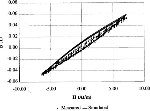
Fig. 4. Comparison of measured, simulated annealing and genetic algorithm
+ simulated annealing BH curves.
[image:3.612.305.551.469.632.2]Fig. 5. Statistical comparison of the performance of the simulated annealing and genetic algorithm approaches for optimization of the Jiles–Atherton magnetic material model.
Fig. 6. Multiple loop optimization results for Siemens N30 (major loop).
V. STATISTICALANALYSIS OFOPTIMIZATIONRESULTS
Although the individual optimization results previously shown are encouraging, due to the random nature of the optimization process in both simulated annealing and genetic algorithm approaches, it is appropriate to investigate the perfor-mance of the respective methods statistically. The optimizations were therefore repeated over a number of runs (20) and the resulting errors compared. The simulated annealing approach was carried out with a variation of 10%, a control factor of 0.001, and 2000 iterations used. The genetic algorithm used 40 generations of a population including 50 individuals (40 times 50 giving a rough equivalent of 2000 iterations). Each generation produced 40 children of whom 20 were mutated. A variation of 20% was introduced in the mutation process. The simulated annealing approach gave a mean value for the error of 0.0219, with a standard deviation of 0.003, while the genetic algorithm gave a mean value for the error of 0.0148, with a standard deviation of 0.009. Fig. 5 shows the histogram of the respective errors for the two methods.
VI. MULTIPLELOOPOPTIMIZATION
[image:4.612.305.553.66.242.2]In practice, for circuit simulation, the resulting optimized model for a magnetic material must be accurate over a wide
Fig. 7. Multiple loop optimization results for Siemens N30 (medium loop).
Fig. 8. Multiple loop optimization results for Siemens N30 (minor loop).
variety of operating conditions. To ensure this is the case, the optimization goal function was extended to allow the optimization of a set of loops rather than a single major loop. Each loop in the set has its own weighting, so if it is essential that the minor loop has a high level of accuracy, but the major loop is not significant, then the weighting can be increased for the minor loop accordingly. An example of this is shown in Figs. 6–8, where the minor loop weighting was set to 5 to improve the relative optimization for the smaller loops. The resulting family of curves show a good match for the minor loop, a reasonable match for the major loop, but a poor match for the medium-sized loops.
VII. CONCLUSION
This paper has demonstrated that it is possible to apply the genetic algorithm technique to the optimization of parameters for the Jiles–Atherton model. It is shown that a small modifica-tion to the Jiles–Atherton model gives an improved matching of
the major loop.
[image:4.612.42.288.262.437.2] [image:4.612.307.551.275.456.2]REFERENCES
[1] D. C. Jiles and D. L. Atherton, “Theory of ferromagnetic hysteresis,” J.
Magn. Magn. Mater., vol. 61, pp. 48–60, 1986.
[2] , “Theory of ferromagnetic hysteresis,” J. Appl. Phys., vol. 55, no. 6, pp. 2115–2120, Mar. 1984.
[3] J. H. Holland, Adaption in Natural and Artificial Systems. Ann Arbor, MI: Univ. Michigan Press, 1975.
[4] D. E. Goldberg, Genetic Algorithms in Search, Optimization and
Ma-chine Learning. Reading, MA: Addison-Wesley, 1986.
[5] Genetic Algorithms in Engineering Systems: Innovations and
Applica-tions. London, U.K.: IEE, Sept. 1997.
[6] P. J. M. Laarhoven and E. H. L. Aarts, Simulated Annealing: Theory and
Applications. Boston, MA: Kluwer, 1989.
[7] D. C. Jiles, J. B. Thoelke, and M. K. Devine, “Numerical determination of hysteresis parameters for the modeling of magnetic properties using the theory of ferromagnetic hysteresis,” IEEE Trans. Magn., vol. 28, pp. 27–35, Jan. 1992.
[8] S. Prigozy, “PSPICE computer modeling of hysteresis effects,” IEEE
Trans. Educat., vol. 36, pp. 2–5, Feb. 1993.
[9] N. Schmidt and H. Güldner, “Simple method to determine dynamic hys-teresis loops of soft magnetic materials,” IEEE Trans. Magn., vol. 32, pp. 489–496, Mar. 1996.
[10] D. Lederer, H. Igarashi, A. Kost, and T. Honma, “On the parameter iden-tification and application of the Jiles–Atherton hysteresis model for nu-merical modeling of measured characteristics,” IEEE Trans. Magn., vol. 35, pp. 1211–1214, May 1999.
[11] F. Preisach, “Über die magnetische nachwirkung,” Zeitschrift Fur
Physik, pp. 277–302, 1935.
[12] P. R. Wilson and J. N. Ross, “Definition and application of magnetic material metrics in modeling and optimization,” IEEE Trans. Magn., submitted for publication.
for the Saber simulator, especially in the areas of power systems, magnetic com-ponents, and telecommunications. His current research interests include mod-eling of magnetic components in electric circuits, VHDL-AMS modmod-eling and simulation, and the development of electronic design tools.
Mr. Wilson is a Member of the IEE and a Chartered Engineer.
J. Neil Ross received the B.Sc. degree in physics from the University of St.
Andrews, St. Andrews, U.K., in 1970 and the Ph.D. degree in 1974 from the same University for his work on the physics of ion laser discharges.
For 12 years, he worked at the Central Electricity Research Laboratories of the CEGB, undertaking research on the physics of high-voltage breakdown and op-tical fiber sensors for use in a high-voltage environment. He joined the Univer-sity of Southampton, Southampton, U.K. in 1987 and has undertaken research in a variety of fields associated with instrumentation and measurement. His current research interests include the modeling of magnetic components for communi-cations, instrumentation, and power applications.
Andrew D. Brown (M’90–SM’96) was born in the United Kingdom in 1955.
He received the B.Sc. degree (with honors) in physical electronics and the Ph.D. degree in microelectronics from Southampton University, Southampton, U.K., in 1976 and 1981, respectively.
He was appointed lecturer in electronics at Southampton in 1981, Senior Lec-turer in 1989, Reader in 1992, and was appointed to an established chair in 1998. He was a Visiting Scientist at IBM, Hursley Park, U.K., in 1983 and a Vis-iting Professor at Siemens NeuPerlach, Munich, Germany, in 1989. He is cur-rently Head of the Electronic System Design Group, Electronics Department, Southampton University. The group has interests in all aspects of simulation, modeling, synthesis, and testing.