Phase singularities in isotropic random waves

Phase singularities in isotropic random waves

By M. V. B er ry a n d M. R. D e n n i s H. H. Wills Physics Laboratory, University of Bristol,

Tyndall Avenue, Bristol BS8 1TL, UK

Received 3 November 1999; accepted 31 January 2000

The singularities of complex scalar waves are their zeros; these are dislocation lines in space, or points in the plane. For waves in space, and waves in the plane (propagating in two dimensions, or sections of waves propagating in three), we calculate some statistics associated with dislocations for isotropically random Gaussian ensembles, that is, superpositions of plane waves equidistributed in direction but with random phases. The statistics are: mean length of dislocation line per unit volume, and the associated mean density of dislocation points in the plane; eccentricity of the ellipse describing the anisotropic squeezing of phase lines close to dislocation cores; distribution of curvature of dislocation lines in space; distribution of transverse speeds of moving dislocations; and position correlations of pairs of dislocations in the plane, with and without their strength (topological charge)§1. The statistics depend on the frequency spectrum of the waves. We derive results for general spectra, and specialize to monochromatic waves in space and the plane, and black-body radiation.

Keywords: phase; dislocations; Gaussian; waves; randomness; singularities

1. Introduction

Phase singularities, that is, dislocations of wavefronts (Nye & Berry 1974; Berry 1981, 1998; Nye 1999)|also called optical vortices|are lines in space, or points in the plane, where the phaseÀ of the complex scalar wave

Á(r; t) =» (r; t) expfiÀ (r; t)g; r=fx; y; zg; (1.1) is unde­ ned. For the generic smooth Á we are interested in, dislocations are also loci of vanishing » : in light, they are lines of darkness; in sound, threads of silence. Interest in optical dislocations has recently revived, largely as a result of experiments with laser ­ elds (Karman et al. 1997; Beijersbergen 1996; Soskin 1997). In low-temperature physics,Ácould represent the complex order parameter associated with quantum ®ux lines in a superconductor or quantized vortices in a super®uid.

This revival prompts us to re-examine that part of the theory dealing with the sta-tistical aspects of dislocations in random waves. Previous studies of these statistics have been restricted to quasimonochromatic paraxial waves (Berry 1978; Baranova

et al. 1981) and experiments and theory for monochromatic waves in two dimensions (Freundet al. 1993; Freund 1994, 1997; Freund & Shvartsman 1994; Freund & Frei-likher 1997; Freund & Wilkinson 1998; Shvartsman & Freund 1994). Here we are able to go further, and calculate analytically statistics describing a variety of geometrical aspects (see x2) of dislocations that need not be monochromatic and that are as

far as possible from paraxial, namely statistically isotropic. Our results will include statistics of dislocation lines for waves propagating in three dimensions, and dislo-cation points for waves in the plane, including, in the latter case, waves propagating in two dimensions and also plane sections of waves propagating in space.

The calculations (seex4) are possible because we employ the model of wave ­ elds as stationary Gaussian random functions (see x3), that is, superpositions of many plane waves with random phases. Important special cases are monochromatic waves (see x5) and black-body radiation (see x6) caricatured by the scalar-wave approx-imation (employed by Rayleigh 1889; Einstein & Hopf 1910a,b). Notwithstanding these results, our treatment is incomplete in several important ways, described inx7. Readers uninterested in the technicalities of the calculations can ignore xx3 and 4.

It will be convenient to separate Áinto its real and imaginary parts,

Á(r; t) =¹ (r; t)+i² (r; t): (1.2) Then dislocations are the intersection lines of the two surfaces

¹ (r; t) = 0; ² (r; t) = 0: (1.3)

All the dislocation statistics we will calculate are gauge invariant in the sense of being unaltered by any smooth (r and t dependent) rede­ nition of phase À , or, equivalently, any smooth rotation in ¹ , ² space.

For the average of any quantity F over the ensemble of random Á, we will use the notation hFi. For waves propagating in two dimensions, and two-dimensional sections of three-dimensional waves, we will use the notation

R² fx; yg; (1.4)

and denote the corresponding gradients by r_R and associated planar averages by su¯ xes 2. We will also use su¯ xes to denote derivatives,

¹ x ² @¹

@x; etc. (1.5)

2. Dislocation geometry

Thecurrent associated with Á is

J= Im(Á¤ rÁ) =» 2rÀ : (2.1)

In the following, a central role will be played by the vorticity associated with J, namely

­ = 1

2r £J = 12Im(rÁ

¤ _{£ rÁ) =r¹ £ r² : (2.2)}

The vector­ is important because it points along the dislocation line. This is because it is perpendicular to the normals to the two surfaces (1.3). Around the dislocation line,À increases by 2º in a positive sense with respect to­ . We will also need the

unit tangent vector talong the dislocation line,

t=­ =!; !² j­ j: (2.3)

For dislocation points in the x; y-plane, the strength Q (also called topologi-cal charge) can be de­ ned (Halperin 1981; Berry 1998) as +1 (¡ 1) if À increases (decreases) by 2º in a positive circuit with respect to e_z,

Q²sgn­ ez = sgn(¹ x² y¡ ¹ y² x): (2.4)

(a) Dislocation densities

The magnitude ! is also the Jacobian determinant transforming ¹ and ² to local coordinates perpendicular to the dislocation, sothe total length of dislocation line in any volume V is

L(V) =

Z

V

dr¯ f¹ (r)g¯ f² (r)g!(r); (2.5)

where here and hereafter dr = dxdydz, and we have not written any time depen-dence explicitly. It follows that the dislocation line density, de­ ned as the mean length of dislocation line per unit volume, is

d=h¯ (¹ )¯ (² )!i=h¯ (¹ )¯ (² )jr¹ £ r² ji: (2.6)

In the plane, the mean number of dislocation lines piercing unit area of a plane is thedislocation point density (cf. Berry 1978),

d2 =h¯ (¹ )¯ (² )j­ ezji=h¯ (¹ )¯ (² )j¹ x² y¡ ¹ y² xji: (2.7)

Both d and d2 have the dimensions (length)¡2. It will be convenient to de­ ne dislocation averages of any quantity f in space or in the plane as

hfid ²

1

dh¯ (¹ )¯ (² )!fi; hfi2;d ²

1

dh¯ (¹ )¯ (² )j¹ x² y¡ ¹ y² xjfi: (2.8)

These select dislocations with weights given by transverse delta-functions, so that volume integrals givef integrated along the dislocations within the volume, correctly weighted by arc length.

(b) Core structure

Around a dislocation line,À changes by 2º , but the change is usually non-uniform (as has been noticed in numerical calculations (Mondragon & Berry 1989)). To under-stand thiscore structure, note ­ rst that, for a dislocation passing throughr=0, the current and amplitude near the dislocation have the forms

J(r)º­ (0)£r for small r;

» 2_{(r)! jr rÁj}2_{º(r r¹ (0))}2_{+(r r² (0))}2 _{for small r;}

)

(2.9)

wherer² jrj. Therefore, the lines ofJare circles enclosing the dislocation (hence the alternative term vortices), and the quadratic form for» 2 _{implies that the local}

con-tours of amplitude are ellipses. These observations are connected with the variation of phase through (2.1), so

rÀ (r)º ­ (0)£r

(r r¹ (0))2 _{+(r r² (0))}2 for small r: (2.10)

Therefore, the polar plot of pjrÀ jaround a circle coaxial with the dislocation is an ellipse with the same eccentricity as the » contours, namely

where¶ § are the eigenvalues of the quadratic form in (2.9). A short calculation gives

¶ § = 1₂

£

(r¹ )2+(r² )2§ p[(r¹ )2_{+(r² )}2_]2_{¡ 4!}2¤_{; (2.12)}

where all quantities are evaluated on the dislocation. Therefore, the eccentricity is

"= p1

2!([(r¹ )

2_{+(r² )}2_]2_{¡ 4!}2₎1=4q_{(r¹ )}2_{+(r² )}2_¡ p_{[(r¹ )}2_{+(r² )}2_]2_{¡ 4!}2_:

(2.13)

We will calculate the spatial and planar core eccentricity averages

h"id and h"i2;d : (2.14)

Freund & Freilikher (1997) calculate two quantities describing the dislocation core structure: the angle betweenÁ_xandÁ_y, and the ratiojÁ_xj=jÁ_yj. Neither is invariant under rotation in thex; y-plane, but taken together they are equivalent to specifying"

and the orientation of the ellipse. In the same paper, a polar plot ofjrÀ jis displayed, corresponding to a curve more complicated than the ellipse generated by pjrÀ j.

(c) Curvature

Dislocation lines are usuallycurved. The curvature is (Eisenhart 1960; do Carmo 1976)

µ(r) =j(t rt)j: (2.15)

We will calculate theprobability distribution of the curvature, which, from (2.3) can be written, after a short calculation, as

P(µ) =h¯ (µ¡ µ(r))i_d = 2µ

d

½

¯ (¹ )¯ (² )!¯

»

µ2¡ jt£(t r)­ j 2

!2

¼ ¾

: (2.16)

(d) Velocity

In waves that are not monochromatic, dislocation lines move. Their transverse velocity v(r; t) (perpendicular to the dislocation lines) is determined by di¬erentiat-ing (1.3), to get

v r¹ =¡ ¹ t; v r² =¡ ² t (2.17)

and then verifying the solution

v(r; t) = (¹ tr² ¡ ² tr¹ )£­

!2 : (2.18)

In three dimensions and in the plane, we will calculate the probability distribution of v=jvj, that is,

P(v) =h¯ fv¡ v(r; t)gi_d = 2vh¯ fv2_{¡ v(r; t)}2_gi

(e) Correlations

Dislocations are not independent random lines in space; their positions are cor-related. The simplest characterization of the correlations is in the plane, where the two simplest non-local statistics can be de­ ned as follows. Let

¹ A²¹ (RA); ¹ B²¹ (RB); RB²RA +R: (2.20)

The pair correlation function g(R) is the mean density of dislocations at position RA+R, given that there is a dislocation at RA, normalized to unity at jRj= 1,

where the dislocations are independent (at least in the statistical model we will use). Thus (cf. equation (2.7))

g(R)² h¯ (¹ A)¯ (² A)¯ (¹ B)¯ (² B)j!Ajj!Bji d2

2

; (2.21)

where now we use the notation

!A =¹ Ax² Ay¡ ¹ Ay² Ax; !B=¹ Bx² By¡ ¹ By² Bx; (2.22)

in which the sign of!is the strength (charge) of the dislocation (cf. equation (2.4)). The pair correlation satis­ es g(R)!1 as jRj ! 1.

Similarly, the charge correlation function gQ(R) (Halperin 1981) gives the

nor-malized density of dislocations separated byR, but weighted with their strengths so that opposite dislocations contribute negatively, that is, equation (2.21) without the modulus signs,

g_Q(R)² h¯ (¹ A)¯ (² A)¯ (¹ B)¯ (² B)!A!Bi d2

2

: (2.23)

Later we will show that the integral of the charge over allR must compensate the charge associated with the dislocation atR =0, that is,

2º d₂

1

0

dR Rg_Q(R) =¡ 1 (2.24)

(of course, this impliesgQ(R)!0 asjRj ! 1). This is a local neutrality condition,

known in the theory of ionic liquids as the ­ rst Stillinger{Lovett sum rule (Stillinger & Lovett 1968a,b). For dislocations, it is the `critical-point screening’ discussed by Freund & Wilkinson (1998). Comparison of !_A and !_B for small R shows that, at the origin, g_Q and g are related by

g(0) =¡ gQ(0): (2.25)

Two other correlation statistics, de­ ned by analogy with useful quantities in the theory of ionic liquids (Hansen & McDonald 1986), are the pair correlations between dislocations of the same strength,g+ + (R), and with opposite strengths,g+ ¡(R). In

terms of g(R) and gQ(R),

3. Gaussian random waves

We consider an ensemble of superpositions of in­ nitely many scalar complex non-dispersive plane waves with speed c,

Á(r; t) =X k

akexpfi[k r¡ ckt¡ ¿ k]g; (3.1)

with wavevectors

k=fk_x; ky; kzg; k² jkj: (3.2)

For waves in the plane, r and k are replaced by R and K = fK_x; Kyg, with K =jKj. Except where otherwise stated, the following holds equally for k andK.

The real amplitudesakare ­ xed, and specify the spectrum of the waves as will be explained soon. The ¿ _k are random phases parametrizing the ensemble. Ensemble averages are averages over 0₆¿ _{k 6}2º for allk, but the functionsÁare ergodic, so ensemble averages are equal to spatial or planar averages.

If the k are suitably dense, any linear combination of the real and imaginary parts (1.2) of (3.1) and their r and t derivatives are stationary Gaussian random functions (Goodman 1985; Rice 1944, 1945 (reprinted in Wax 1954)), whose central properties will now be stated for future reference. Consider any set of N functions

u(r; t) = fu₁(r; t): : : uN(r; t)g; (3.3)

in which eachunis¹ or² or any of their derivatives, and any set of auxiliary variables

b=fb₁: : : b_Ng: (3.4)

Then

hexpfib u(r; t)gi= expf¡ 1 2h(b u)

2_{ig= expf¡} 1

2b M bg; (3.5)

whereM is the matrix of correlations

(M)_mn=hu_mu_ni: (3.6)

Using (2.5), theprobability density of u(r; t) can easily be found,

P(u)² h¯ fu¡ u(r; t)gi

= 1

(2º )N

Z

db expf¡ ib ughexpfib u(r; t)gi

= expf¡

1 2u M

¡1 _ug

(2º )N=2p_detM : (3.7)

Before usingP(u) to calculate the geometrical averages of x2, it is necessary to determine the correlationsM(equation (3.6)), involving averages of products of pairs of un. Explicit averaging over ¿ k in (3.1) shows that all such quadratic averages are of the form

hf(k)i= 1 2

X

k

Now we make the central speci­ cation that the randomness of the waves we are considering is isotropic, so that a_k depends only on the length k, and de­ ne the

radial power spectrum ¦ by 1

2

X

k

a2_kf(k)²

Z

dk¦ (k)

4º k2f(k) (three dimensions);

1 2

X

K

a2_Kf(K)²

Z

dK ¦ 2(K)

2º K f(K) (two dimensions):

9 > > > = > > > ; (3.9)

For plane sections of waves in three dimensions,¦ and¦ 2are related by projection

in wavevector space,

¦ 2(K) = 2º K

Z 1

¡1

dkz

¦ (pk2 z+K2)

4º (k2 z +K2)

=K

Z 1

K

dk ¦ (k)

kpk2_{¡ K}2: (3.10)

Multiplication of¦ by a constant corresponds to rescaling the strength of the wave Á and leaves all dislocation averages una¬ected. It is convenient to normalize ¦ to unity, that is,

Z 1

0

dk ¦ (k) = 1;

Z 1

0

dK ¦ 2(K) = 1; (3.11)

so that the fundamental averages are

h¹ 2i=h² 2i= 1: (3.12)

For radial averages and radial moments, it will be convenient to use the notation

Z 1

0

dk f(k)¦ (k)² hhfii; hhkm_{ii ²k}

m; (3.13)

and similarly in the plane, indicated by the subscript 2 and with K replacingk. The quadratic averages needed to calculate the dislocation statistics ofx2 are of two sorts. First, with ¬ denoting x, y or z, there are products of u_¬ at the same position and time; of these, the only non-zero products are

h¹ 2

¬ i=h² ¬2i=¡ h¹ ¹ ¬ ¬ i=¡ h² ² ¬ ¬ i= 1₃k2; h¹ _¬2i2 =h² ¬2i2 = 1₂K2;

h¹ 2

¬ ¬ i=h² ¬ ¬2 i= 15k4; h¹ 2

¬ ­i=h² ¬ ­2 i=h¹ ¬ ¬ ¹ ­ ­i=h² ¬ ¬ ² ­ ­i= ₁₅1 k4 (¬ 6=­); h¹ 2

ti=h² t2i=c2k2; h¹ ² _ti=¡ h² ¹ _ti=ck1:

9 > > > > > > > > > = > > > > > > > > > ; (3.14)

Second, there are products involving di¬erent positions. These occur in the planar correlation statistics (2.21) and (2.23). The fundamental averages of this non-local type are (cf. equation (2.20))

C(R)² h¹ _A¹ Bi=h² A² Bi=hhJ0(K R)ii2=

½ ½

sin(kR)

kR

¾ ¾

de­ ning the autocorrelation function C(R), and where the last equality applies to plane sections of waves propagating in space. To write the remaining zero non-local averages, we can choose the x-axis to lie along the direction of the vector R=RB¡ RA. Then

h¹ _A¹ Bxi=h² A² Bxi=¡ h¹ Ax¹ Bi

=¡ h² Ax² Bi=¡ hhKJ1(K R)ii2²C0(R); h¹ _Ax¹ Bxi=h² Ax² Bxi=¡ hhK2J000(KR)ii2=¡ C00(R);

h¹ _Ay¹ Byi=h² Ax² Byi=

1

RhhKJ1(KR)ii2 =¡

C0_(R)

R :

(3.16)

All other relevant averages, local and non-local, are zero. Note, in particular, that all averages involving both¹ and ² vanish, excepth¹ ² _ti=¡ h² ¹ _ti.

Our calculations will be for general radial power spectra¦ . However, the following are important special cases. For monochromatic waves propagating in space and in the plane, the respective spectra are densities on a spherical shell ink space and on a ring in K space:

¦ (k) =¯ (k¡ k0); ¦ 2(K) =¯ (K¡ K0): (3.17)

Forplane sections of monochromatic waves in space, we have, from (3.10), the pro-jection of the sphere spectrum

¦ 2(K) =

K£ (k0¡ K) k₀ k2

0¡ K2

; (3.18)

where £ denotes the unit step. For black-body radiation with temperature T, and thermal wavenumber de­ ned by

kT ² kBT

~c ; (3.19)

wherekBis Boltzmann’s constant, the radial (Planck) spectrum is

¦ (k) = 15k

3

º 4_k4

T[exp(k=kT)¡ 1]

: (3.20)

4. Calculation of averages for general spectra

In calculating averages, we make use of the joint probability density of the magnitude of vorticity !and the gauge-invariant quantity

G² jrÁj2= (r¹ )2+(r² )2: (4.1) As shown in Appendix A, the three-dimensional distribution is

P(!; G) = 27! 2k3 2

exp ¡ 3G

2k2

£ (G¡ 2!); (4.2)

and, in the plane,

P2(!; G) =

2

K2 2

exp ¡ G K2

(a) Dislocation densities

For the line density (2.6), we note that all quantities in the average are indepen-dent, so

d= 1 2º

Z 1

0

dG

Z 1

0

d! !P(!; G): (4.4)

With (4.2), the integral is elementary, and gives

d=k₂=3º : (4.5)

For the point density (2.7), a similar argument based on (4.3) gives

d2 =K2=4º : (4.6)

If Á in the plane is a section of a wave in space, equation (3.10) applies, and gives

K2= 2₃k2; (4.7)

whence

d₂= 1

2d: (4.8)

In this result, the 1

2 is the spherical average of the factorjcos³ jrelating contributions

todandd2from lines making angles ³ with the normals to the faces of a unit cube.

(b) Dislocation core structure

For the core eccentricity, we require the averages (2.14), involving !2 _{and G. In}

three dimensions, using (2.13), (4.2) and (4.5), and rescaling G,

h"i_d = 81 4p2

Z 1

0

dG

Z G=2

0

d! !expf¡ 3

2Gg(G2¡ 4!2)1=4

q

G¡ pG2_{¡ 4!}2_{: (4.9)}

With the substitution != 1

2uG, theGintegral is trivial, and theuintegral can also

be evaluated, leading to

h"id =

3º

8p2 = 0:8330: (4.10)

In the plane, analogous calculations give

h"i_2;d = 2p2

Z 1

0

dG

Z G=2

0

d!expf¡ Gg(G2¡ 4!2)1=4

q

G¡ pG2_{¡ 4!}2_{; (4.11)}

leading to

h"i_2;d = p3

2sinh

¡1_{1¡ 1 = 0:8697: (4.12)}

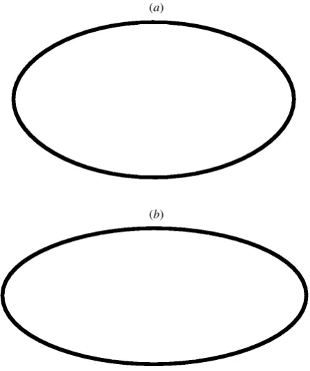
These eccentricities are rather large (­ gure 1), showing that the typical phase struc-ture is strongly anisotropic. Note that the eccentricities are independent of the spec-tra ¦ and ¦ 2; they are universal numbers characterizing the dislocation cores of

(a)

(b)

Figure 1. Ellipses representing anisotropy of phase structure near dislocation cores. (a) Transverse to dislocations in space. (b) In the plane.

(c) Dislocation curvature

For the curvature (2.16), calculations are greatly simpli­ ed by evaluating the derivatives of­ in local coordinates whosez-axis is along­ . Then

µ(r)2 = (@z« x)

2 _+(@ z« y)2 !2

= 1

!2(¹ 2

zz(r² )2+² zz2 (r¹ )2¡ 2¹ zz² zzr¹ r² ): (4.13)

The only non-diagonal correlation matrix (cf. equations (3.3) and (3.6)) is

M= ± 1 ¡ 13k2 ¡ 1

3k2 15k4 ²

for u=f¹ ; ¹ _zzg; (4.14)

whence

P(¹ = 0; ¹ zz) =

1

2º µ_cpk₂exp

»

¡ ¹ 2 zz

2µ2 ck2

¼

; (4.15)

whereµc is the characteristic curvature

µc ²

s

9k4¡ 5k22

45k2

From (2.16), we need to calculate the dislocation average

P(µ) = µ

º

Z 1

¡1

dq expf¡ iqµ2ghexpfiqµ(r)2gi_d ; (4.17)

where µ2 _{is given by (4.13). The averages over ¹}

zz and ² zz now involve a

two-dimensional complex Gaussian integral. In evaluating this, and also the trivial aver-ages over ¹ and ² , it is convenient to transform to the scaled curvature

µ_{s c}² µ µc

; P(µ) = 1

µc

P(µ_{s c}); (4.18)

and also to rescale !and G. Then we ­ nd, after substituting ford from (4.5),

P(µ_{s c}) = 3µs c 2º

Z 1

¡1

dq expf¡ iqµ2 s cg

½ _! p

D(!; G; q)

¾

; (4.19)

whereD, the determinant from the Gaussian integration, is

D(!; G; q) = 1¡ 2iqG

!2 ¡ 4 q2

!2: (4.20)

Some non-obvious manipulations are required to apply (4.2) to the evaluation of the triple integral in (4.19) (over q, !and G). These are explained in Appendix B.

The result is

P(µs c) =

35=2_µ s c

(µ2

s c+3)5=2

: (4.21)

All moments diverge except the ­ rst two, which are

hµi_d =p3µ_c; hµ2_i

d = 6µ2c: (4.22)

(d) Dislocation speed

We use (2.18) and (2.19); the squared speed is

v(r; t)2₌ 1 !2[¹

2

t(r² )2+² 2t(r¹ )2¡ 2¹ t² tr¹ r² ]: (4.23)

The only non-diagonal correlation matrices are

M§ =

³

1 §ck1

§ck1 c2k2

´

foru+ =f¹ ; ² _tg; u¡=f² ; ¹ tg; (4.24)

whence

P(¹ = 0; ² _t) = 1 2º vc

p k2

exp

»

¡ ² 2 2

2v2 ck2

¼

(4.25)

(and similarly for ² , ¹ t), wherevc is the characteristic speed

vc²c

q

(1¡ k2

This is for three dimensions; for waves propagating in the plane,k1 and k2 must be

replaced by K1 and K2, and we denote the characteristic speed by vc2.

The complete formal similarity between (4.23), (4.25) and (4.13){(4.15) in the curvature calculation means that the speed distribution in three dimensions can be written by analogy with (4.21), after rescaling to the dimensionless speed

vs c² v vc

; P(v) = 1

vc

P(vs c): (4.27)

The distribution is

P(v_{s c}) = 3

5=2_v s c

(v2

s c+3)5=2

: (4.28)

All moments diverge except the ­ rst two, which are

hvid = p

3vc; hv2id = 6v2c: (4.29)

In the plane, the analogous result, obtained with the aid of (4.3) rather than (4.2), is

P2(vs c) =

4v_{s c}

(v2 s c+2)2

: (4.30)

Only the ­ rst moment does not diverge,

hvi_{d ;2}= pº

2vc2: (4.31)

As written, equations (4.30) and (4.31) apply to waves propagating in the plane. For plane sections of waves propagating in space,vc2 must be replaced by the

three-dimensional vc of (4.26) (because, for such sections, !=ck, not cK).

It is important to note that the speeds v in the spatial and planar distribu-tions (4.28) and (4.30) can take any value from zero to in­ nity: v is not limited by the common speed cof the dispersionless waves in the superposition (3.1). This is not a violation of relativity, because dislocations are forms rather than things (like searchlight beams and intersections of scissor blades): no energy moves with them (because they are zeros) and they cannot be used to transmit information. In fact, it is possible to construct simple exact solutions of the dispersionless wave equation possessing single dislocations moving with arbitrary speed (Nye & Berry 1974).

(e) Dislocation correlations

For the pair correlation (2.21), we eliminate the modulus signs using the identity

j!j= 1

º

Z 1

¡1

dt

t2(1¡ cos(!t)): (4.32)

Thus (2.21) becomes

g(R) = 1

d2 2º 2

Z 1

¡1

dtA t2

A

Z 1

¡1

dtB t2

B

[T(0;0)¡ T(tA;0)¡ T(tB;0) + 1

where

T(tA; tB) =h¯ (¹ A)¯ (² A)¯ (¹ B)¯ (² B) expfi(!AtA¡ !BtB)gi: (4.34)

The merit of this substitution is that since the ! depend quadratically on ¹ and ² , the average in (4.34) will involve only a Gaussian integral.

There are two non-diagonal correlation matrices, since, from (3.16), the two vectors

u₁=f¹ _A; ¹ _B; ¹ _Ax; ¹ _Bxg; u₂=f¹ _Ay; ¹ _Byg (4.35) are independent (and similarly for correlations involving ² ). With the notations

C ²C(R); E ²C0(R); H² ¡ C0(R)=R; F ² ¡ C00(R); F0² ¡ C00(0) = 1₂K2;

(4.36)

the matrices corresponding tou1 andu2 are

M1 =

1 C 0 E

C 1 ¡ E 0

0 ¡ E F0 F

E 0 F F₀

; M₂= F0 H

H F0

: (4.37)

We need

detM1²D1= [E2¡ (1+C)(F0¡ F)][E2¡ (1¡ C)(F0+F)];

detM2²D2=F02¡ H2:

(4.38)

Then the relevant probability densities are

P(¹ A= 0; ¹ B= 0; ¹ Ax; ¹ Bx) =

expf¡ 1 2u

0

1 N1 u01g

(2º )2_D 1

;

P(¹ Ay; ¹ By) =

expf¡ 1

2u2 N2 u2g

(2º )2_D 2

;

(4.39)

where

u0₁ ² f¹ _Ax; ¹ Bxg;

N1 =

1

D1

¡ [E2_{¡ F}

0(1¡ C2)] cE2¡ F(1¡ C2) cE2_{¡ F(1¡ C}2_{) ¡ [E}2_{¡ F}

0(1¡ C2)] ;

N2 =

1

D₂

F0 ¡ H ¡ H F0

;

(4.40)

and similarly for ² .

The average (4.35) is now an eight-dimensional complex Gaussian integral whose evaluation gives

T(tA; tB) =

1 (2º )2_D(t

A; tB)

where

D(tA; tB) = (1¡ C2)2+(t2A+t2B)F0(E2¡ F0(1¡ C2))

¡ tAtBH(CE2¡ F(1¡ C2))+t2At2BD1D2: (4.42)

Now, after scaling tA andtB, the pair correlation (4.33) becomes

g(R) = F0(E

2_{¡ F}

0(1¡ C2))

4º 4_d2

2(1¡ C2)2

Z 1

¡1

dtA t2

A

Z 1

¡1

dtB t2

B

I(tA; tB; Y; Z); (4.43)

where

Y ² H

2_(CE2_{¡ F(1¡ C}2₎₎2 F2

0(E2¡ F0(1¡ C2))2

; Z² D1D2(1¡ C 2₎

F2

0(E2¡ F0(1¡ C2))2

(4.44)

and

I(t_A; t_B; Y; Z) = 1¡ 1

1+t2 A

¡ 1

1+t2 B

+ 1+t 2

A+t2B+Zt2At2B

(1+t2

A+t2B+Zt2AtB2)2¡ 4Y t2At2B

: (4.45)

Because I is a rational function, the tA integral can be evaluated by residues,

leaving, after integrating by parts overtBand substituting ford2from (4.6), the pair

correlation

g(R) = 2(E

2_{¡ F}

0(1¡ C2)) º F₀(1¡ C2₎2

Z 1

0

dt3¡ Z +2Y +(3+Z¡ 2Y)t

2_+2Zt4

(1+t2₎3p_{1+(1+Z¡ Y)t}2_+Zt4 : (4.46)

It is possible to express this as an explicit, but very complicated, combination of elliptic integrals, that we do not write. In any case, the integral converges very well and is easy to evaluate numerically.

For the charge correlation (2.23), the absence of modulus signs makes the eval-uation much easier, since the average can be expressed as derivatives of Gaussian integrals involving the probability densities (4.39). The result, expressed using the notation (4.36), is

gQ(R) =

2E(CE2_{¡ F(1¡ C}2₎₎ RF2

0(1¡ C2)2

= 1

F2 0R

@R

³ _E2_(R)

1¡ C2_(R)

´

: (4.47)

The ­ rst equality is a special case of a formula previously obtained by Halperin (1981). The second equality, together withE(0) = 0, leads immediately to the screen-ing relation (2.24).

We can get further insight into critical-point screening by considering the charge

Q(N) associated with the dislocations within an area A = N=d2, where the mean

number of dislocations isN (N ¾1). Obviously, the average chargehQ(N)iis zero. But what about the mean square ®uctuation hQ2_{(N)i? If the charges merely have}

average neutrality, there are no long-range correlations, and we expecthQ2_{(N)i ¹ N.}

An exact calculation (with the boundary of A Gauss-smoothed to eliminate trivial edge e¬ects) gives (for all N)

hQ2_(N)i= 1 2N

±

1+2º d2

Z 1

0

dR RgQ(R) exp

»

º R2

2A

¼ _²

= 1 2N

±

1+2º d2

Z 1

0

dR RgQ(R) ²

+1 2d22º 2

Z 1

0

dR R3_g

Q(R)+O(N¡1):

Without critical-point screening, the leading term is the ­ rst one, and the ®uctuations are those of a random distribution with overall neutrality. But for dislocations, there is screening, and the ­ rst term vanishes, leaving ®uctuations that are independent of N for large N. Further manipulation gives

hQ2_(A)i= 1

8

Z 1

0

dR R2@R

µ

C0(R)2

1¡ C2_(R)

¶

+O(N¡1): (4.49)

5. Monochromatic waves

For monochromatic waves in space with wavenumber k0 = 2º =¶ , the spectrum

is (3.17), and so the dislocation line density (4.5) is

d= k

2 0

3º : (5.1)

For a plane section of the same wave, the density (4.6) of dislocation points is

d2= k2

0

6º =

2º

3¶ 2: (5.2)

A measure of the spacing of these points is

1

p d2

= 0:691¶ : (5.3)

The characteristic curvature (4.16) is µ_c = 2k₀=p45, so the curvature averages (4.22) are

hµ2_i

d = 2hµi2d = 158k 2

0: (5.4)

A measure of the radius of curvature is

1=phµ2_{i= 0:218¶ ; (5.5)}

indicating that dislocations are rather sharply curved on the wavelength scale. For the pair and charge correlation statisticsg(R) and gQ(R), we need the

auto-correlation function (3.15),

C(R) = sin(k0R)

k0R

: (5.6)

Figure 2 shows g(R) and gQ(R), calculated from (4.46) and (4.47). At the origin, g(0) =¡ g_Q(0) = 2

5, showing modest repulsion between dislocations.

For monochromatic waves in the plane, with wavenumber K₀ = 2º =¤ with ring spectrum (3.17), the density of dislocation points is

d₂= K

2 0

4º =

º

¤ 2: (5.7)

A measure of the spacing of these points is

1.0

0.75

0.25 0.50

- 0.25

10R

g

,

gQ

2 4 6 8

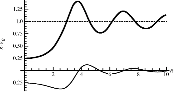
Figure 2. Correlation statistics for a plane section of monochromatic waves in space, in units ofk0. Thick line: pair correlationg(R). Dashed line: asymptotic valueg= 1. Thin line: charge correlationgQ(R).

The autocorrelation function (3.15) is

C(R) =J0(K0R); (5.9)

from which the pair and charge correlations can be calculated (­ gure 3). At the origin, g(0) =¡ gQ(0) = 1=4, indicating a stronger repulsion between dislocations.

Note that, except very close to the origin, there is no obvious relation between

g and gQ. Now, the strength Q (equation (2.4)) alternates between neighbouring

dislocations on the net formed by the intersections of zero lines of¹ and² ; this is the `sign principle’ (Freund & Shvartsman 1994). Thus one might expect that alternate maxima ofg(`rings’ of dislocations) would correspond to maxima and minima of g_Q

(representing oppositely charged rings of dislocations). But the topological relation seems not to have a metrical counterpart. We have checked this by calculating g

and gQ for a `blurred’ square lattice, of alternating dislocations whose vertices are

randomly displaced according to a Gaussian distribution; if the blurring becomes comparable with the lattice spacing, there is again no relation between g and gQ.

The only vestige of the sign principle in the charge correlations (Shvartsman & Freund 1994) seems to be the fact thatgQ(0) is negative (cf. equation (2.25)).

Of course, for monochromatic waves the dislocations do not move.

6. Black-body radiation

With the spectrum (3.20), involving the thermal wavenumber (3.19), the wavenumber moments (3.13) are

kn=

15

º 4k n

T(n+3)!± (n+4); k1= 3:832kT;

k2= 40₂₁º 2k2T; k4= 8º 4k4T;

9 > > > > > = > > > > > ;

1.0 1.25

0.75

0.25 0.50

- 0.25

10R

g

,

g Q

2 4 6 8

Figure 3. Correlation statistics for monochromatic waves in the plane, in units ofK0. Thick line: pair correlationg(R). Dashed line: asymptotic valueg= 1. Thin line: charge correlationgQ(R).

so the dislocation line density (4.5) is

d= 40 63º k

2

T: (6.2)

For a plane section of the same wave, the density (4.6) of dislocation points is

d2= 20₆₃º k2T =

80º 3

63¶ 2 T

; (6.3)

where ¶ _T = 2º =kT is the thermal wavelength. A measure of the spacing of these points is

1=pd2= 0:159¶ T: (6.4)

This seems rather small, but it should be noted that ¶ T does not correspond to the

maximum of the Planckk-distribution (3.20); this lies atk= 2:831kT, corresponding

to a wavelength 0:354¶ T.

The curvature statistics (4.22) are

hµ2_i

d = 2hµi2d = 59381575k 2

T: (6.5)

A measure of the radius of curvature is

1=phµ2i= 0:026¶ T; (6.6)

indicating that (even though ¶ T is not the maximum of the Planck distribution)

dislocations are even more sharply curved than in the monochromatic case (5.5), showing the e¬ect of large wavenumbers in the Planck distribution.

For the characteristic speed (4.26), equations (6.1) give vc = 0:468c, whence the

moments (4.29) of the transverse speed are

p hv2

d i= p

- 1.0

- 0.5

- 1.5 1.0 1.5

0.5

1R

g

,

gQ

0.2 0.4 0.6 0.8

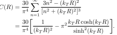
Figure 4. Correlation statistics for a plane section of black-body radiation, in units of the thermal wavenumberkT. Thick line: pair correlation g(R). Dashed line: asymptotic valueg = 1. Thin line: charge correlationgQ(R).

For the pair and charge correlation statistics g(R) andg_Q(R), we need the autocor-relation function (3.15). This can be calculated as

C(R) = 30

º 4

1

X

n= 1

3n2_{¡ (k} TR)2

[n2_+(k TR)2]3

= 30

º 4

µ ₁

(kTR)2

¡ º 2kTRcosh(kTR)

sinh2(k_TR)

¶

: (6.8)

Figure 4 shows g(R) and gQ(R), calculated from (4.46) and (4.47). At the origin, g(0) =¡ g_Q(0) = 3=2, showing considerable clustering (anti-repulsion) between dis-locations, notwithstanding the topological sign repulsion.

7. Concluding remarks

We have calculated some statistics that describe the geometry of dislocation lines in complex scalar Gaussian random waves in two and three dimensions. In this, the wave equation played only a minor role|restricting the time dependence of the plane-wave constituents, and so a¬ecting the calculations of speed. Apart from this, the results apply to any complex scalar random functions, not just the waves that are our main interest.

The geometry thus revealed is extraordinarily complicated and occasionally coun-terintuitive: dislocations sharply curved on the wavelength scale, moving faster than light, and with positions correlated in ways apparently unrelated to the topological alternation of sign. Nevertheless, much remains to be understood, both mathemati-cally and physimathemati-cally.

For local statistics, a fully three-dimensional characterization requires understand-ing of thetorsionas well as the curvature. Preliminary investigation suggests that the mean-square torsion diverges and the distribution of torsion has a long tail, indicat-ing that dislocations are typically locally helical rather than ®at rindicat-ings. For non-local statistics, the correlations g and gQ are just the start of an in­ nite hierarchy of N

of dislocations. More interesting are global, that is, topological, statistics. We can ask: are dislocation lines typically closed in space? Can they be knotted? If knotted, what is the distribution of knot invariants (Adams 1994)? Since (as it is easy to show by example) pairs of dislocations can be linked, what is the distribution of linking numbers? If higher-order links are possible (e.g. Borromean triples (Cromwell et al. 1998)), what is the distribution of numbers characterizing such links?

Finally, we mention the application to black-body radiation. Given the importance of black-body radiation in physics, it is a little surprising that its detailed geometric structure has not been fully understood. Here we have made some progress, but as a physical model, the scalar-wave approximation is inadequate. Better would be an understanding of the singularities of the electromagnetic ­ eld of black-body radia-tion, but it is not clear what the relevant singularities are|the vector singularities studied so far (Nye 1983a,b, 1999; Nye & Hajnal 1987) are restricted either to paraxial or monochromatic waves, and so are inapplicable here. We are studying this question now.

We are grateful to Dr John Hannay for many helpful suggestions and to Professor Isaac Freund for a useful correspondence. M.V.B.’s research is supported by The Royal Society; in addition, he thanks the Lorentz Institute of the University of Leiden for generous hospitality while writing the ¯rst draft of this paper. M.R.D. is supported by a University of Bristol postgraduate scholarship.

Appendix A. Joint probability distribution of ! and G

De­ ning the 3-vectors a = r¹ , b = r² and a = jaj, b= jbj, we have, from (2.2), (2.3) and (4.1),

P(!; G) =h¯ (!¡ ja£bj)¯ (G¡ a2_{¡ b}2_{)i: (A 1)}

All components ofaandbare independent, so the matrix of correlations is diagonal and, using (3.14) and polar coordinates for aandb, with thez-axis forbalong a,

P(!; G) = 27

º k3 2

Z 1

0

da a2

Z 1

0

db b2

Z º

0

d³ sin³

£exp

»

¡ 3(a 2_+b2₎

2k2

¼

¯ (!¡ absin³ )¯ (G¡ a2_{¡ b}2_{): (A 2)}

With the successive changes of variable

a=» cos¿ ; b=» sin¿ ; ¿ = 1

2® ; sin³ sin® =s; sin® =t; (A 3)

evaluation is straightforward though tedious, and gives (4.2).

The planar calculation, in which a and b are 2-vectors, proceeds similarly, and gives (4.3).

Appendix B. Curvature and speed integrals

We outline the calculation for curvature in three dimensions; for speed in three dimensions, the calculation is identical, and for speed in the plane the arguments are very similar. With (4.2), equation (4.19) becomes

P(µ_{s c}) = 81µs c 4º

Z 1

¡1

dq expf¡ iqµ2 s cg

Z 1

0

dGexpf¡ 3 2Gg

Z G=2

0

d! !

2

p

Changing to variables

!= 1

2G· ; q=G» (B 2)

eliminates G from D and enables theGintegral to be evaluated, to give

P(µs c) =

243µs c

4º

Z 1

0

d· · 3

Z 1

¡1

d» _p 1

· 2_{¡ 8i» ¡ 16»} 2₍3

2 +i» µ2s c)5

: (B 3)

The » integrand contains a pole and two branch points, which can be connected by a cut. The contour can be deformed around the cut without passing through the pole, and then the further transformations

» = 1

4i(v¡ 1); · = p

u (B 4)

lead to

P(µs c) =

15 552µs c

º

Z 1

0

du u

Z 1

¡1

dvp 1

1¡ v2_(6+µ2

s c¡ µ2s cv p

1¡ u)5: (B 5)

Use of

Z 1

¡1

dv p

1¡ v2_(a+v)5 =

º (3+24a2_+8a4₎

8(a2_{¡ 1)}9=2 (B 6)

leads to a uintegral that is elementary, leading eventually to (4.21).

References

Adams, C. C. 1994The knot book. San Francisco, CA: Freeman.

Baranova, N. B., Zel’dovich, B. Y., Mamaev, A. V., Pilipetskii, N. & Shkukov, V. V. 1981 Dislocations of the wavefront of a speckle-inhomogeneous ¯eld (theory and experiment).JETP Lett.33, 195{199.

Beijersbergen, M. 1996 Phase singularities in optical beams. Thesis, Huygens Laboratory, Leiden. Berry, M. V. 1978 Disruption of wavefronts: statistics of dislocations in incoherent Gaussian

random waves.J. Phys.A11, 27{37.

Berry, M. V. 1981 Singularities in Waves and Rays. InLes Houches lecture series(ed. R. Balian, M. Kl¶eman & J.-P.Poirier), vol. 35, pp. 453{543. Amsterdam: North-Holland.

Berry, M. V. 1998 Much ado about nothing: optical dislocation lines (phase singularities, zeros, vortices, : : : ). In Proc. Int. Conf. on Singular Optics (ed. M. S. Soskin), SPIE vol. 3487, pp. 1{15.

Cromwell, P., Beltrami, E. & Rampicini, M. 1998 The Borromean rings. Mathematical Intelli-gencer 20, 53{62.

do Carmo, M. P. 1976 Di® erential geometry of curves and surfaces. Englewood Cli® s, NJ: Prentice-Hall.

Einstein, A. & Hopf, L. 1910a On a theorem of the probability calculus and its application to the theory of radiation.Ann. Phys.33, 1096{1104.

Einstein, A. & Hopf, L. 1910b Statistical investigation of a resonator’s motion in a radiation ¯eld.Ann. Phys.33, 1105{1115.

Eisenhart, L. P. 1960A treatise on the di® erential geometry of curves and surfaces. New York: Dover.

Freund, I. 1997 Critical-point level crossing geometry in random wave ¯elds.J. Opt. Soc. Am. 14, 1911{1927.

Freund, I. & Freilikher, V. 1997 Parameterization of anisotropic vortices.J. Opt. Soc. Am.A14, 1902{1910.

Freund, I. & Shvartsman, N. 1994 Wave-¯eld phase singularities: the sign principle.Phys. Rev.

A50, 5164{5172.

Freund, I. & Wilkinson, M. 1998 Critical-point screening in random wave ¯elds. J. Opt. Soc. Am.A15, 2892{2902.

Freund, I., Shvartsman, N. & Frehlikher, V. 1993 Optical dislocation networks in highly random media.Opt. Commun.101, 247{264.

Goodman, J. W. 1985Statistical optics. Wiley.

Halperin, B. I. 1981 Statistical mechanics of topological defects. InLes Houches lecture series

(ed. R. Balian, M. Kl¶eman & J.-P. Poirier), vol. 35, pp. 813{857. Amsterdam: North-Holland. Hansen, J.-P. & McDonald, I. R. 1986Theory of simple liquids. Academic.

Karman, G. P., Beijersbergen, M. W., van Duijl, A. & Woerdman, J. P. 1997 Creation and annihilation of phase singularities in a focal ¯eld.Optics Lett.22, 1503{1505.

Mondragon, R. J. & Berry, M. V. 1989 The quantum phase 2-form near degeneracies: two numerical studies.Proc. R. Soc. Lond.A424, 263{278.

Nye, J. F. 1983a Lines of circular polarization in electromagnetic wave ¯elds. Proc. R. Soc. Lond.A389, 279{290.

Nye, J. F. 1983b Polarization e® ects in the di® raction of electromagnetic waves: the role of disclinations.Proc. R. Soc. Lond.A387, 105{132.

Nye, J. F. 1999 Natural focusing and ¯ne structure of light: caustics and wave dislocations. Bristol: Institute of Physics Publishing.

Nye, J. F. & Berry, M. V. 1974 Dislocations in wave trains.Proc. R. Soc. Lond.A336, 165{190. Nye, J. F. & Hajnal, J. V. 1987 The wave structure of monochromatic electromagnetic radiation.

Proc. R. Soc. Lond.A409, 21{36.

Rayleigh, Lord 1889 On the character of the complete radiation at a given temperature.Phil. Mag.27, 460{469.

Rice, S. O. 1944 Mathematical analysis of random noise.Bell. Syst. Tech. J.23, 282{332. Rice, S. O. 1945 Mathematical analysis of random noise.Bell. Syst. Tech. J.24, 46{156. Shvartsman, N. & Freund, I. 1994 Wave¯eld phase singularities: near-neighbour correlations and

anticorrelations.J. Opt. Soc. Am.A112710{2718.

Soskin, M. S. (ed.) 1997Proc. Int. Conf. on Singular Optics, SPIE, vol. 3487.

Stillinger, F. H. & Lovett, R. 1968aIon-pair theory of concentrated electrolytes. I. Basic con-cepts.J. Chem. Phys.48, 3858{3868.

Stillinger, F. H. & Lovett, R. 1968bGeneral restriction on the distribution of ions in electrolytes.

J. Chem. Phys.49, 1991{1994.

By M. V. B e rr y a n d M. R. D en n is

Proc. R. Soc. Lond. A456, 2059{2079 (2000)

Corrigendum 1. Equation (4.48) and the material to the end of _x3 should be

replaced by

hQ2(N)_i= 1₂N 1+2º d2

1

0

dR RgQ(R) exp ¡

º R2

2A

= 1

4

1

0

dR R C0(R) 2

(1_¡ C(R)2₎exp ¡ º R2

2A ; (4.48)

where in deriving the second equality we have used equation (4.47) and the critical-point screening relation (2.24) that follows from it. The ­ rst equality shows that without critical-point screening, the leading term for large N would be 1

2N, and the

®uctuations would be those of a random distribution with overall neutrality. But for dislocations there is screening, and

hQ2(N)_i= 1

4

1

0

dR R C0(R) 2

1_¡ C2_(R) +O(N

¡1_{); (4.49)}

provided the integral converges, leaving ®uctuations that are independent of N for largeN. However, for the sharp spectra representing monochromatic waves in space ((3.17) and (5.6) later), and in the plane ((3.18) and (5.9) later), the integral does not converge. Then we can show from (4.48) that _hQ2_{(N)i ¹ logN for waves in}

space, and_hQ2_{(N)i ¹} p_{N for waves in the plane.}

Corrigendum 2.Equation (6.8) should be replaced by

C(R) = 30

º 4

1

n= 1

3n2_{¡ (k}

TR)2 [n2 _+(k

TR)2]3

= 15

(º k_TR)4 1¡ (º kTR)

3 cosh(º kTR) sinh3(º kTR)