Efficient Algorithms For The Inference Of Minimum Size DFAs

°

Efficient Algorithms for the Inference of Minimum

Size DFAs

ARLINDO L. OLIVEIRA [email protected]

JO ˜AO P. M. SILVA [email protected]

IST-INESC/Cadence European Labs, R. Alves Redol 9, Lisboa, Portugal

Editors: Vasant Honavar and Colin de la Higuera

Abstract. This work describes algorithms for the inference of minimum size deterministic automata consistent with a labeled training set. The algorithms presented represent the state of the art for this problem, known to be computationally very hard.

In particular, we analyze the performance of algorithms that use implicit enumeration of solutions and algorithms that perform explicit search but incorporate a set of techniques known as dependency directed backtracking to prune the search tree effectively.

We present empirical results that show the comparative efficiency of the methods studied and discuss alternative approaches to this problem, evaluating their advantages and drawbacks.

Keywords: deterministic finite automata, implicit enumeration, search methods

1. Introduction and related work

This work addresses the problem of inferring a finite automaton with minimum size that matches a labeled set of input strings. This problem has been extensively studied in the literature, both from a practical and theoretical point of view.

Selecting the minimum DFA consistent with a set of labeled strings is known to be NP-complete. Specifically, Gold (Gold, 1978) proved that given a finite alphabet6, two finite subsets S,T ⊆ 6∗ and an integer k, determining if there is a k-state DFA that recognizes L such that S ⊂L and T ⊂6∗−L is NP-complete. Furthermore, it is known

that even finding a DFA with a number of states polynomial on the number of states of the minimum solution is NP-complete (Pitt & Warmuth, 1993).

If all strings of length n or less are given (a uniform-complete sample), then the problem can be solved in time polynomial on the size of the training set (Porat & Feldman, 1988). Note, however, that the size of the input is in itself exponential on the number of states in the resulting DFA. Angluin has shown that even if an arbitrarily small fixed fraction(|6(n)|)², ² >0 is missing, the problem remains NP-complete (Angluin, 1978).

an interesting approach that does not require the availability of a reset signal to take the automaton to a known state.

All these algorithms address simpler versions of the problem discussed here where we assume the learner is given a set of labeled strings and is not allowed to make queries or experiment with the automaton. The basic search algorithm for this problem was pro-posed by Biermann (Biermann & Feldman, 1972). Later, the same author propro-posed an improved search strategy that is much more efficient in the majority of the complex prob-lems (Biermann & Petry, 1975). Section 5.1 describes these algorithms in detail. More recently, the applicability of implicit enumeration techniques to this problems was studied (Oliveira & Edwards, 1996). These techniques are analyzed in Section 4.

One contribution of this work is the demonstration that advanced search techniques can be applied to this inference problem, improving the efficiency of the search algorithms by several orders of magnitude. More specifically, we show how the application of dependency-directed backtracking techniques improves significantly the search algorithm proposed by Biermann. These techniques, applied to date in other domains like truth maintenance systems (Stallman & Sussman, 1977) and boolean satisfiability solvers (Silva, 1995), allow the search algorithm to prune large sections of the search tree by diagnosing the ultimate causes of conflicts encountered during the search. In many cases, these conflicts are caused by assignments that were made several levels above and significant parts of the search tree can be removed from consideration. These techniques are described in Section 5.2.

The algorithms described are evaluated in a set of problems with known solutions. The results presented in Section 6 show that some of the algorithms described actually extend the scope of applicability of the search techniques and make the algorithms able to handle many problems of non-trivial size.

A different approach is to view the problem of selecting the minimum automaton con-sistent with a set of strings as equivalent to the problem of reducing an incompletely specified finite automaton. This problem is more general than the one addressed here and was also proved to be NP-complete by Pfleeger (Pfleeger 1973). However, previous work (Oliveira & Edwards, 1996) has shown that these algorithms are extremely inefficient when applied to this problem, and present no advantages over the approaches presented here.

Other techniques have been proposed for the inference of finite state automata, some of them based on recurrent neural network architectures (Giles et al., 1992; Pollack, 1991). Although these methods may exhibit, from a conceptual standpoint, some advantages, published results (Horne & Giles, 1995) show that neural network based methods are not competitive in inference problems where the exact identification of the minimum finite state automaton is the objective at hand.

2. Motivation

In fact, heuristic methods for this problem that aim at selecting a small but not necessarily minimum size solution have been proposed and met considerable success (Lang et al., 1998). The most successful approaches to date are based on the idea of merging states that are compatible (Trakhtenbrot & Barzdin, 1973; Oncina & Garcia, 1992; Lang, 1992). These methods, commonly known as Evidence Driven State Merging (EDSM) algorithms, can be made to run in polynomial time if no backtrack or only limited backtrack is allowed. Furthermore, it is known that if the learning set includes a characteristic set (Oncina & Garcia, 1992) whose size is quadratic on the size of the target DFA, then these algorithms return the exact solution to the problem. In many situations, however, it is impossible to enforce the presence of a characteristic set. In this case, the algorithms can still be applied, but without the warranty of convergence to the global optimum solution.

When this is the case, several mergings are possible, but only some choices will lead to the optimum solution. A number of heuristic approaches has been proposed to guide the search process (Juill´e & Pollack, 1998), leading to a set of algorithms that have been remarkably successful solving problems of significant complexity (Lang et al., 1998). Given the known complexity of the problem, it is likely that the induction of large DFAs can only be accomplished when heuristic methods as these are used. However, it is well known that, as the size of the labeled training set gets smaller, methods that do not perform search lose the ability to identify DFAs of a size comparable with the minimum solution and become ineffective as a method to infer accurate classification rules for strings (Lang et al., 1998).

It turns out that, in many domains, the size of the available training set is the dominating factor, and exact determination of the minimum DFA consistent with the training set is the most promising approach for the inference of the desired target hypothesis. This is usually the case whenever human intervention is required to perform the labeling of the examples in the training set. Although the methods described here have a specific application domain in mind, similar restrictions on the size of the training set will exist in other domains, making, in some situations, exact methods the best choice. We therefore believe that the algorithms presented here are highly relevant to the machine learning community, even outside the particular domain under consideration.

The particular domain we are concerned with is digital circuit design and, more specif-ically, the synthesis of a finite state controller from descriptions of observed input/output signals. We assume the designer has available a set of waveforms describing input/output relationships, and is interested in deriving a finite state controller that generates those waveforms. Sets of waveforms represent a very natural way for circuit designers to repre-sent protocols, and are commonly used to specify properties and characteristics of a variety of digital devices.

In general, the designer is interested in a finite state controller that not only generates the waveforms presented, but also behaves correctly in a variety of similar, but distinct, conditions. Under certain general conditions, it is possible to obtain such a controller without providing all possible input/output waveforms. To achieve this goal, we first transform the set of waveforms specified by the designer into a DFA with output of a particular type, a

loop-free DFA (LFDFA), formally defined in the next section. Intuitively a LFDFA is a

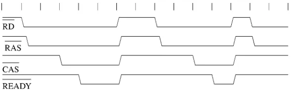
Figure 1. Sample waveforms for a dynamic memory controller.

The goal of deriving the desired finite state controller can then be achieved by selecting the DFA with minimum number of states that is equivalent to this LFDFA.

To exemplify the task at hand, consider the waveforms shown in figure 1. They represent the waveforms that should be generated by a dynamic memory controller (RAS,CAS, READY) in response to a read request from the processor or cache controller (RD). It

is clear that these particular waveforms can be generated by the Mealy type LFDFA1shown in figure 2.

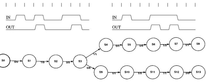
This is valid in general for any set of input/output waveforms that start at a known reset state. If instead of a single waveform we have a set of waveforms, all starting at a known reset state, we obtain a tree like state transition graph, as shown in figure 3.

Clearly, the LFDFAs generated directly from the set of input/output waveforms provided are of limited utility as a specification of the desired controllers, because they will not be able to generate the control signals in situations that do not match exactly the waveforms present in the traces.

Although we will not address in detail the arguments over the merit of the Occam’s razor approach (Blumer et al., 1987), we argue that the selection of a minimum size DFA compatible with this specification is the method most likely to yield the desired result. In fact, a variety of results show that there is a strong correlation between the complexity of the generated hypothesis (Peark, 1978; Blumer et al., 1986; Li & Vit´anyi, 1994) and the probability of obtaining a controller that implements the desired behavior. In the example

Figure 3. Traces and loop free DFA for a modulus 2 counter.

Figure 4. Minimal size DFA for the memory controller.

shown above, the minimum DFA compatible with the waveforms in figure 1 is shown in figure 4. This finite state controller generates not only control signals compatible with the waveforms shown in figure 1, but also captures the essence of the protocol intended by the designer. Clearly, for this method to be reliable, the process of providing waveforms and generating the finite state controller has to go through several iterations, with the designer providing additional details at each iteration. However, the details of this procedure are outside the scope of this work, since here we are specifically concerned with algorithms that efficiently generate the automaton in figure 4 from the automaton in figure 2.

Other applications may also require exact solutions for the problem of finding mini-mum states DFAs compatible with given LFDFAs. Recently, one of the authors proposed a methodology for the reduction of states in finite state controllers that uses, as a subroutine, an exact method for the reduction of LFDFAs (Pena & Oliveira, 1998).

3. Problem definition

3.1. Basic definitions

Definition 1. A deterministic finite automaton (DFA) is a Mealy model finite state au-tomaton represented by the tuple M =(6, 1,Q,q0, δ, λ)where6 6= ∅is a finite set of

input symbols, 1 6= ∅ is a finite set of output symbols, Q 6= ∅is a finite set of states,

q0 ∈ Q is the initial “reset” state,δ(q,a): Q×6 → Q∪ {φ}is the transition function,

andλ(q,a): Q×6 →1∪ {²}is the output function.

We will assume that Q = {q0,q1, . . . ,qn}and will use q∈ Q to denote a particular state, a ∈ 6 a particular input symbol and b ∈ 1a particular output symbol. For Moore type DFAsλ(q,a1)=λ(q,a2)for all a1,a2 ∈ 6. For Moore type DFAs with a binary output

alphabet, a state is considered an accepting state if the output is 1, and non-accepting if the output is 0. In the sequence, we will consider that the DFAs are of the Mealy type, although the methods can be directly applicable to Moore type DFAs.

An automaton is incompletely specified if the destination or the output of some transition is not specified. When referring to incompletely specified automata, we will useφto denote an unspecified transition and²to denote an unspecified output. The functionδ(q,a)defines the structure of the state transition graph of the automaton while the functionλ(q,a)defines the labels present in each of the edges of that graph.

We say that an output biis compatible with an output bj (and write bi ≡bj) if bi =bj

or bi =²or bj =².

The domain of the second variable of functionsλandδ is extended to strings of any length in the usual way.

Definition 2. The output of a sequence s =(a1, . . . ,ak)applied to state q,denoted by

λ(q,s),represents the output of an automaton after a sequence of inputs(a1, . . . ,ak),is

applied in state q. The output of such a sequence is defined to be

λ(q,s)=λ(δ(δ(· · ·δ(q,a1)· · ·),ak−1),ak) (1)

Definition 3. The destination state of a sequence s =(a1, . . . ,ak),denoted byδ(q,s),

represents the final state reached by an automaton after a sequence of inputs(a1, . . . ,ak),

is applied in state q. This state is defined to be

δ(q,s)=δ(δ(. . . δ(δ(q,a1),a2) . . .),ak) (2)

To avoid unnecessary notational complexities,λ(φ,a)=²andδ(φ,a)=φ, by defini-tion.

3.2. Training sets and loop free automata

The objective is to infer an automaton with minimum number of states that is consistent with a given training set. A training set is specified by one or more sequences of input-output pairs:

Definition 4. A training set is a set of pairs T = {(s1,l1), . . . , (sm,lm)}where each pair

Accepted: 1 11 1111 Rejected: 0 101

Figure 5. Training set specified as a set of accepted and rejected strings.

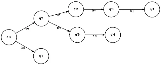
Figure 6. Loop free automaton for the example training set shown.

If the output alphabet is the set{0,1}the training set can be viewed as specifying a set of accepted strings (the ones that output 1) and a set of rejected strings (the ones that output 0). We will say that T contains a string s if(s,l)is in T and l6=². An example of a possible training set is given in figure 5.

Alternatively, the training set can be specified by one or more sequences where, at each time, the value of the input/output pair is known. Both forms of training set descriptions are equivalent and can be viewed as defining a particular type of incompletely specified automata, a Loop Free Automata (LFDFA). A LFDFA is a DFA that has a state transition graph without loops or re-convergent paths. Figure 6 shows the LFDFA that corresponds to the training set in figure 5.

There is a one to one correspondence between loop free automata and training sets. A loop free automaton represents a training set iff

1. Its output for each input sequence present in the training set agrees with the label in that training set.

2. The output for input sequences not present in the training set is undefined.

Formally,

Definition 5. An automaton is said to be the loop free automaton representing a training set T if it satisfies Definition 1 and the following additional requirements:

∀q ∈ Q\q0,∃1(qi,a)∈ Q×6 s.t. δ(qi,a)=q ∀q ∈ Q,∀a∈6 δ(q,a)6=q0

λ(q0,si)=li if(si,li)∈T,

These requirements specify that there exists one and only one (symbol∃1) string that, when applied at state q0makes the automaton reach state q and that state q0is not reachable

from any other state. This is the same as saying that the graph that describes the LFDFA is a tree rooted at state q0.

Since the training set T defines uniquely the corresponding loop-free automaton, we will use T to denote both the training set itself and the LFDFA that it defines. We will in general use quoted symbols (Q0,δ0, etc) to refer to the loop free automata and unquoted symbols to refer to the resulting completely specified automata that is the result of the algorithm.

The aim is to construct an automaton M that exhibits a behavior equivalent to T , that is, an automaton M that outputs the same output as T every time this output is defined.

Definition 6. An automaton M = (6, 1,Q,q0, δ, λ)is equivalent to a LFDFA T =

(6, 1,Q0,q₀0, δ0, λ0)iff, for any input string s=(a1, . . . ,ak) λ(q0,s)≡λ0(q00,s).

Given a specific mapping function F : Q0→ Q with F(q₀0)=q0from the states in T to

the states in M, it defines a valid solution iff it satisfies the following two requirements:

Definition 7. A function F satisfies the output and transition requirements iff:

∀q = F(q0), λ0(q0,a)≡λ(q,a) (3)

∀q = F(q0),F(δ0(q0,a))=δ(q,a) (4)

It is known that the minimum finite state automaton that satisfies the training set can be found by selecting an appropriate mapping function that maps the states in T to the states in M.

Let T =(6, 1,Q0,q₀0, δ0, λ0)be an LFDFA and M = (6, 1,Q,q0, δ, λ)be a

com-pletely specified DFA. Consider now a relation F between the states of T and the states of

M defined as follows:

Definition 8. Let F : Q0 → Q be defined by F(δ0(q₀0,s)) = δ(q0,s)for each string s

contained in T .

In these conditions, the following lemma applies:

Lemma 1. F is a many to one mapping, mapping each state in T to one and only one state in M.

Proof: since T is an LFDFA each state in T can be reached by one and only one string. Therefore, the definition of F will assign a unique state in M to each state in T . 2

Theorem 1. Let T be a LFDFA. Then, for any automaton M compatible with T , the function F as defined above is a valid mapping function between the states of T and the states of M.

Proof: Since M is equivalent to T , it gives an output compatible with T , for every string

and assume that F(q0)=q becauseδ0(q₀0,s)=q0andδ(q0,s)=q (definition of F ). Now,

λ0_(q0_,a)=λ0_(q0

0,sa)≡λ(q0,sa)=λ(δ(q0,s),a)=λ(q,a), and therefore equation 3 is

respected. On the other hand, F(δ0(q0,a))=F(δ0(q_o0,sa))=δ(q0,sa)=δ(δ(q0,s),a)=

δ(q,a)=δ(F(q0),a)and therefore equation 4 is also respected. Therefore, F is a mapping function satisfying equations (3) and (4). 2 This result has been implicitly used by Biermann (Biermann & Petry, 175) and a slightly different proof has been presented in Oliveira and Edwards (1996). Is is important to note that, in general, the minimum DFA equivalent to a given incompletely specified DFA can

not be obtained by selecting a mapping function in this way. This result is only valid for

LFDFAs, not for generic DFAs (Pena & Oliveira, 1998).

Since any automaton that satisfies these requirements can be found by selecting a mapping function, the objective of selecting the minimum consistent DFA can be attained by selecting a mapping function that exhibits a range of minimum cardinality.

For the sake of simplicity, we follow Biermann’s original notation and will define Si as

the index of the state in the target automaton that state q_i0in the original LFDFA maps to, i.e., qSi =F(qi0)(Biermann & Petry, 1975).

An equivalent DFA with N states can therefore be found by selecting an assignment to the variables S0, . . . ,Sn, such that each Si is assigned a value between 0 and N−1, and

this assignment defines a mapping function that satisfies (3) and (4).

3.3. Compatible and incompatible states

Two states q_i0and q0_jin a finite state automaton T are incompatible if, for some input string

s,λ(q_i0,s)6≡λ(q0_j,s). This information can be represented by a graph, the incompatibility

graph. The nodes in this graph are the states in Q0, and there is an edge between state q_i0 and q0_jif these states are incompatible.

The incompatibility graph is represented by a function I : Q0×Q0→ {1,0}. I(q_i0,q0_j)

is 1 if and only if states q_i0and q0_jare incompatible.

A clique in the incompatibility graph gives a lower bound on the size of the minimum automaton. By definition, pairs of incompatible states cannot be mapped to the same state and therefore, a clique in this graph corresponds to a group of states that must map to different states in the resulting automaton. Identifying the largest clique in a graph is in itself an NP-complete problem (Garey & Johnson, 1979). A large clique (not necessarily the maximum one) can be identified using a slightly modified version of a well known exact algorithm (Carraghan & Pardalos, 1990). The size of the clique provides a lower bound on the number of states needed in the resulting automaton. This lower bound is used as the starting point for the search algorithms described in the next section. If the algorithms described in the next section fail to find an automaton with a number of states equal to the lower bound, we increase N by one and re-execute the algorithms.

3.4. DFA inference as a constraint satisfaction problem

satisfaction problem (CSP). The constraints that need to be obeyed by the mapping function are the following:

1. If two states q_i0and q0_jin the original LFDFA are incompatible, then Si 6=Sj.

2. If two states q_i0and q0_j have successor states q_k0 and q_l0for some input u, respectively, then Si =Sj ⇒Sk=Sl.

These two conditions can be rewritten as:

I(q_i0,q0_j)=1 ⇒ Si 6=Sj (5)

and

q_k0 =δ0¡q_i0,a¢∧q_l0=δ0¡q0_j,a¢ ⇒ Si 6=Sj ∨Sk=Sl (6)

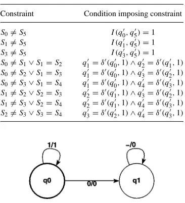
For any given training set, equations (5) and (6) will generate a set of restrictions that have to be obeyed in order to generate a valid solution. As an example, consider the training set considered in figure 5 and the corresponding LFDFA in figure 6. The constraints generated by this training set are shown in Table 1.

In this case, it is trivial to verify by inspection that the following assignment will provide a solution of minimum cardinality: S0 =S1=S2=S3 =S4=0 and S5 =S6=S7 =1.

Once the mapping is obtained, the generation of the minimum inferred DFA inferred is straightforward. There will be one state for each value in the range of the mapping function, and transitions will be labeled in accordance with the transitions specified in the LFDFA. In this example, this mapping generates the minimum DFA shown in figure 7.

Table 1. Subset of constraints generated from the training set in figure 5. Constraint Condition imposing constraint S06=S5 I(q00,q05)=1 S16=S5 I(q01,q05)=1 S36=S5 I(q03,q05)=1 S06=S1∨S1=S2 q10 =δ0(q00,1)∧q20 =δ0(q01,1) S06=S2∨S1=S3 q10 =δ0(q00,1)∧q30 =δ0(q02,1) S06=S3∨S1=S4 q10 =δ0(q00,1)∧q40 =δ0(q03,1) S16=S2∨S2=S3 q20 =δ0(q10,1)∧q30 =δ0(q02,1) S16=S3∨S2=S4 q20 =δ0(q10,1)∧q40 =δ0(q03,1) S26=S3∨S3=S4 q30 =δ0(q20,1)∧q40 =δ0(q03,1)

One may think that, given that the problem can be posed as a CSP, a general purpose CSP solver would be able to perform this optimization task in an efficient way. However, our experiments with a number of existing CSP solvers have shown that this is not the case. General purpose CSP solvers are too general to be efficient in this particular problem, and we had no success applying them to this task. One must note that the set of constraints generated by even a relatively small training set is extremely large, a factor that seems to strongly limit the performance of general purpose CSP solvers.

Other authors have also realized that the DFA inference problem can be stated as a CSP problem (Coste & Nicolas, 1998). The approaches described in this work follows a similar formulation, but the search methods proposed to solve it are significantly different.

The two algorithms described in the following sections can also be viewed as CSP solvers, but they have been specifically designed for this problem, and therefore perform much more efficiently. In fact, they trade efficiency for generality. General CSP solvers are able to accept more general constraints, but that generality has a severe impact of the complexity of their internal data structures and on their efficiency on this particular problem.

4. Implicit search algorithms

Recent research in the field of logic synthesis (Coudert, Berthet & Madre, 1989) and discrete optimization (Kam et al., 1994) has shown that implicit enumeration algorithms can be very effective in dealing with search problems with extremely large search spaces. Implicit enumeration algorithms are based on the idea of replacing the explicit search for a solution by a description, in implicit form, of a function describing all the possible solutions.

The implicit approach described in this section follows that philosophy and avoids the need to explicitly search for the right mapping function. It does so by keeping an implicit description of all the mapping functions that satisfy the output and transition requirements. This approach makes the implicit algorithm very simple to describe, but incurs the over-head imposed by the use of discrete function manipulation primitives. This overover-head can be recovered if the regularities of the problem make the use of an implicit enumeration technique more efficient than an explicit one.

To simplify the explanation, we assume that the output alphabet 1is equal to the set

{0,1}. The approach can be easily applied to the more general case.

4.1. Discrete functions and multi-valued decision diagrams

The discrete function manipulation needed to keep this implicit list of possible mappings is performed using multi-valued decision diagrams to represent the discrete functions involved. A full description of this technique is outside the scope of this work and only a brief introduction is made here. The reader is referred to Kam & Brayton (1990) for a more complete treatment. Any binary valued function of k discrete variables, x1,x2, . . . ,xk

F : P1×P2× · · · ×Pk→ {0,1} (7)

variable. An MDD for F has two terminal nodes nzand nothat correspond to the leaves of

the graph. Every non-terminal node ni, labeled with variable xj, has|Pj|outgoing edges

labeled with the possible values of xj. Each of these edges points to one child node. The

value of F for any point in the input space can be computed by starting at the root and following, at each node, the edge labeled with the value assigned to the variable tested at that node. The value of the function is 0 if this path ends in node nz and 1 if it ends in

node no.

A decision diagram is called reduced if no two nodes exist that branch exactly in the same way and it is never the case that all outgoing edges of a given node terminate in the same node (Bryant, 1986). A decision diagram that is both reduced and ordered is called a reduced ordered decision diagram. For a given variable ordering, reduced, ordered MDDs are canonical representations for functions defined over that domain.

Packages for the manipulation of discrete functions using MDDs allow the user to realize (Kam & Brayton, 1990), amongst others, the following operations:

1. Creation of a function from an arithmetic relation. For example, f :=(xi =xj)returns

the function that is 1 for all points of the input space where xi =xj.

2. Boolean combination of existing functions. For example, f :=g∧h returns the function

that is 1 only when functions g and h are 1.

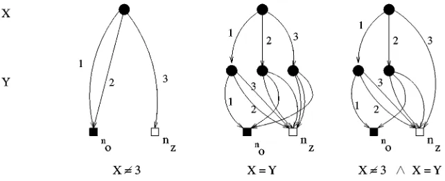
As an example, figure 8 depicts the MDDs for the functions f :=(x6=3), g :=(x =y)

and h := f ∧g, all defined over P×P, P = {1,2,3}.

4.2. Implicit enumeration of solutions

The objective is to satisfy the constraints expressed in Section 3.4 using as few values as possible for the values of Si in equations (5) and (6). The idea is to keep an implicit list

of the valid solutions to this CSP that can be directly manipulated using simple Boolean operations. This list is kept by considering a function F:{0, . . . ,N −1}|Q0| _{→ {0,1}}

defined as follows:

Definition 9. F(S0,S1, . . . ,S|Q0|−1)=1 for the pointv0, v1, . . . , v|Q0|−1 if the mapping

function F defined by S0 =v0,S1 =v1, . . . ,S|Q0|−1 =v|Q0|−1 corresponds to a mapping

function satisfying constraints (5) and (6).

A solution of the CSP described in Section 3.4 can now be found in a trivial way by simply computing the MDD representation of the following expression

F¡S0,S1, . . . ,S|Q0|−1

¢

= ^

i,j s.t. I(q_i0,q0_j)=1 Si6=Sj

^

k,l,i,j s.t. q_k0=δ0(q_i0,a)∧q_l0=δ0(q0_j,a)

Si 6=Sj∨Sl =Sk (8)

where the domain of each Si(and therefore, of each MDD variable) ranges from 0 to N−1,

where N is the current target for a solution of the constraint satisfiability problem. Note that the actual implementation of this expression involves two rather trivial iteration loops, since the MDD manipulation package internally handles all the operations on the MDDs. However, the actual computation of the MDD representing expression 8 may require extensive amounts of memory and computation, even if the final solution can be represented by an MDD with a small number of nodes. If there are only k solutions with size N , it is guaranteed that the MDD representing those solutions will not have more than k|Q0|nodes (Oliveira et al., 1998). However, MDDs resulting from intermediate computations can have an exponentially higher number of nodes, representing the bottleneck of this computation.

4.3. Ordering and other efficiency issues

There are two important ordering problems to be addressed in the algorithm. The first one is the order in which states are processed when expression (8) is computed. The experiments have shown that no other ordering improved significantly the performance when compared with the ordering obtained by performing a breadth first search in the graph that represents T . This is the ordering used, by default.

The second ordering that deserves consideration is the ordering in which variables are stored internally in the MDD package. The best results were obtained by sorting the states according to the degree of the respective nodes in the incompatibility graph.

5. Explicit search algorithms

5.1. The basic search algorithm

The explicit search algorithm for the solution of the CSP posed in Section 3.4 searches for a solution for the constraints (5) and (6) by constructing a search tree and backtracking whenever some partial assignment is found to lead to a contradiction. When looking for an automaton with N states, the basic search with backtrack procedure iterates through the following steps:

2. Extend the current assignment by selecting a value from the range 0. . .N −1 and assigning it to S. If no more values exist, undo the assignment made to the last variable chosen.

3. If the current assignment leads to a contradiction, undo it and goto step 2. Else goto step 1.

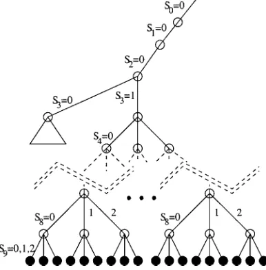
This search process can be viewed as a search tree (or decision tree). We define the decision level as the level in this tree where a given assignment was made. The assignment made at the root is at decision level 0, the second assignment at decision level 1, and so on. To illustrate the fundamental differences between this and succeeding search techniques, consider an hypothetical example where a search is being performed by an automaton with 3 states. Under these conditions, each Si can assume only the values 0, 1 or 2. Suppose

that variables will be assigned in the order S0,S1, . . . ,S9and that the following constraints

exist in this problem:

S1 6=S2∨S8=S9 (9)

S8 6=S9∨S2=S3 (10)

The section of the search tree depicted in figure 9 is obtained by the basic search algorithm described above. In every leaf of this tree a conflict was detected and backtracking took place.

Biermann noted (Biermann & Petry, 1975) that a more effective search strategy can be applied if some bookkeeping information is kept and used to avoid assigning values to variables that will later prove to generate a conflict. This bookkeeping information can also

be used to identify variables that have only one possible assignment left, and should therefore be chosen next. This procedure can be viewed as a generalization to the multi-valued domain of the unit clause resolution of the Davis-Putnam procedure (Davis & Putnam, 1960), and can be very effective in the reduction of the search space that needs to be explored.

This can be done in the following way2

• For each node in q0_j ∈ Q0, a table is kept that lists the values that Sjcan take.

• Every time some Si is assigned to the value z, the tables for all unassigned nodes are

updated according to the following algorithm:

– If I(q_i0,q0_j)=1, then z is removed from the list of values that Sjcan be assigned to.

(Equation (5))

– If the assignment of Siforces some specific value z on some node ql0(forced by equation

(6)), then all values except z are removed from the table of possible values in node q_l0.

• When selecting the next variable Si to assign, priority is given to the variables that

correspond to nodes in Q0that can at that depth take only one possible value.

Clearly, the information on these tables needs to be updated after every assignment is made to some Si and also after each backtrack takes place. Biermann has shown, and our

experiments have confirmed, that for hard problems, this improved search strategy leads to considerable improvements in speed, and expands the size of the problems that can be addressed.

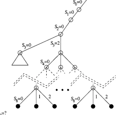
For the example considered above, the section of the search tree obtained is shown in figure 10. Note that as soon as a value is assigned to S8, the algorithm automatically identifies

that no solution exists because no value can possibly be assigned to S9. This may lead to very

considerable savings, specially if S9is not the next variable to be assigned. The search tree

obtained by this algorithm is qualitatively different because many nodes have a branching factor equal to 1 and the order by which assignments are performed is no longer fixed.

5.2. Explicit search using dependency directed backtracking

In this section, we show that the application of recently developed search techniques can improve considerably the efficiency of the search algorithm and extend the range of problems that can be effectively solved. In particular, these techniques will avoid the need to explicitly search all the replicated subtrees that are present in the search tree shown in figure 10.

The improvement proposed is the application of conflict diagnosis techniques to allow for the use of dependency directed backtracking. In this paper, we use the term dependency

directed backtracking to denote two techniques that can, in fact, be used independently.

The first technique is based on the realization that, under certain conditions, it is possible to perform jumps in the decision tree that span one or more decision levels. These jumps are called non-chronological backtracks or backjumps (Russel & Norvig, 1996). The second technique is based on the fact that, under similar conditions, it is possible to assert a set of constraints that need to be obeyed in the future if a solution is to be found.

Before we describe these techniques, we will first reformulate slightly the problem at hand. For this, we point out that the set of constraints (5) and (6) can be computed only once at the beginning of the algorithm execution. This means that a set of constraints is generated, where each constraint is of the form:

(X1op X2)∨(X3op X4)∨ · · · ∨(Xn₋1op Xin) (11)

Each constraint is a disjunction of one or more elements of the form Xiop Xi+1where

each Xi is either a variable Sj or a constant in the range 0 to N −1. Each operator op is

either=or6=. Constraints generated from equation (5) have one element, while constraints generated from equation (6) have 2 elements. It is clear that the algorithm can be easily extended to satisfy any constraints with more than 2 elements, but the problem formulation does not create them.

Conflict diagnosis (Silva & Sakallah, 1996) is a technique first proposed by Stallman and used in the context of truth-maintenance systems (de Kleer, 1986) and constraint satisfia-bility solvers (Stallman & Sussman, 1977). To make clear how conflict diagnosis can be used to prune the search tree, consider again the example described above, and the section of the search tree shown in figure 11. In this problem, for each possible value assigned to

S8, a conflict is detected as soon as all the values of S9 are considered. In this example

the conflicts detected in the backtrack points A, B and C can be traced to the following conditions: a) S1=S2and b) S26=S3. Under these conditions, all the possible assignments

to S8and S9failed to yield a solution, and therefore no solution can be found until one of

these assignments is removed. This fact has two immediate consequences:

1. No progress can be made by assigning other values to S4, S5up to S7, until at least one

Figure 11. Example of non-chronological backtracking used by the improved search algorithm (BIC).

2. If the conditions that caused this conflict, namely the specific assignments made to S1, S2and S3, are again present in some other part of the search tree, they will generate a

replica of this conflict.

Therefore, we can state that the current assignments to S1, S2and S3can not be present in

any assignments that lead to a solution. This means that we can perform a non-chronological backtrack to the decision level where S3was assigned and that a new constraint can be added

to the constraints in the database.

These facts lead to the following general procedure for handling conflicts and controlling the backtrack search procedure.

1. Every time a conflict is detected, diagnose the conflict and generate a constraint that expresses that conflict. The result of this diagnosis is the consensus of all the assignments that originated the conflict.

2. Identify the variable present in the conflict that is at the highest decision level, and perform a non-chronological backtrack to that level.

3. Store the constraint generated by the conflict diagnosis engine in the constraint database, and use it to restrict choices of variables in the future. This is usually described as

dependency directed backtracking.

5.3. Conflict diagnosis

in a constraint of the form of the general constraint (11). Consider again the example in figure 11, and the conflicts detected in nodes A, B and C. At each of these nodes, it is found that no possible assignments exist to variable S9.

Analyzing in more detail the conflict in node A, we see that S9 cannot take the value

0 because the second constraint in the example, constraint (10) is not satisfied, given the current assignments S2 =0 and S3=1. The other values possible for S9, 1 or 2, are barred

because constraint (9) would not be satisfied, since S1 =0 and S2 =0. The condition that

leads to this conflict can therefore be written as:

S1=0∧S2=0∧S3=1∧S8=0 (12)

This condition represents simply the consensus of all the constraints that lead to the conflict in this node. The last element in the constraint, S8=0 is also a cause of the conflict, and

therefore should be listed in the condition.

For nodes B and C, a similar procedure could be followed and we would arrive at the following two conditions:

S1 =0∧S2=0∧S3=1∧S8 =1 (13)

S1 =0∧S2=0∧S3=1∧S8 =2 (14)

Note that, in this simplified example, the three conditions are very similar, but that needs not be the case in general. The cause of the conflict detected in node D can now be diagnosed as the consensus of the causes of all the conflicts in the children nodes, A, B and C. The consensus of a set of constraints is simply the conjunction of all constraint elements that are in agreement in all the constraints in the set. A variable that is present in all the values of its domain is removed. In this case, all the values for variable S8were tried, and therefore

the conflict cannot be due to any specific choice of S8. This is a general rule, and a

non-chronological backtrack can only be made after all the possible choices for a given variable have been tried.

The conflict in node D is therefore diagnosed as being caused by

S1=0∧S2=0∧S3=1 (15)

To solve this conflict, the negation of this condition has to be asserted, and therefore the constraint

S16=0∨S26=0∨S36=1 (16)

can be added to the database, since this constraint will have to be satisfied in any assignments that lead to a solution.

This leads to the following general procedure for the diagnosis of conflicts and control of backtrack:

1. At each leaf in the search tree, compute the set of assignments involved in the conflict. 2. At each non-leaf node where a conflict is detected, compute the consensus of all the

conditions involved in the conflicts of children nodes.

3. Complement the resulting condition, and add it to the constraint database. Also, store this condition as the cause of the conflict at this node.

4. Compute the highest decision level involved in this condition, and perform a non-chronological backtrack to that level.

6. Experimental results

6.1. Performance comparison of the algorithms

To test the performance of the algorithms described in Sections 4, 5.1 and 5.2, we used a randomly generated set of 115 Mealy type finite state automata with binary inputs and outputs. These finite state automata were reduced and unreachable states were removed before the experiments were run. The size of the automata (after reduction) varied between 3 and 19 states. A total of 575 training sets were generated, with each training set containing twenty strings of length 30. Each program was given 30 minutes of CPU time and 128 Megabytes of memory to find the minimum consistent automaton in a 133 MHz Pentium running Linux.

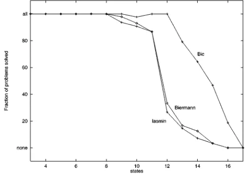
Of the total of 575 problems, Biermann’s approach (described in Section 5.1) solved 371, the implicit algorithm (Iasmin) described in Section 4 solved 363, and the explicit search algorithm improved with dependency directed backtracking (Bic) managed to solve 468. The graph in figure 12 shows the fraction of problems that are solved by each algorithm,

plotted as a function of the number of states in the finite state automaton that represents the solution.Bicmanages to solve the large majority of the problems that have a solution with no more than 12 states, while the other approaches start failing for problems with solutions between 9 and 10 states. At first glance, it may seem that this difference is relatively small and easily due to small differences in implementation details. However, that turns out not to be the case. In fact, the problems with 12 states are several orders of magnitude harder to solve, not only because the search space is much larger, but also because the training set is, relatively speaking, much sparser. In fact, the advantage ofBicover the other two approaches can be as large as several orders of magnitude.

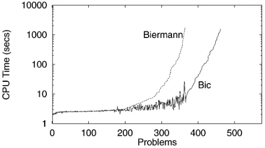
Figure 13 shows the total CPU time spent byBicand Biermann’s original algorithm, while figure 14 compares the CPU time ofBicagainstIasmin. In both cases, the problems were sorted in order of increasing CPU time taken by the algorithms.

Figure 13. Comparison of the CPU time spent by Biermann’s algorithm andBic, the explicit search algorithm with dependency directed backtracking.

It is interesting to note that the behavior of Biermann’s algorithm and the implicit search method implement inIasmingive very comparable results. This happens despite the fact that Biermann’s algorithm andIasminsearch the solution space using radically different approaches. However,Iasminrequires considerably more memory than Biermann’s ap-proach, which basically requires an amount of memory linear on the size of the original training set.

We have no clear idea why these two different algorithms perform so similarly in this set of problems. Clearly, the intrinsic difficulty of this task when the DFA sizes approach 10 states justifies partially the similar results, but a more detailed analysis of the characteristics of this problem is required to fully understand the reasons behind this phenomenon.

6.2. Analysis of the advantages of dependency directed backtracking

It is interesting to analyze how the use of dependency directed backtracking improves, in a systematic way, the performance of the algorithm. For that, we performed a comparison of the number of backtracks performed by Biermann’s algorithm andBic.

Figure 15 shows the number of backtracks required for each problem. It is clear that the number of backtracks used byBicis much smaller than the number of backtracks used by Biermann’s approach. However, each backtrack takes longer to execute in the modified algorithm. Figure 16 shows the time each backtrack takes to execute, for all the problems that are solved in the alloted time. This graph shows that, in the interesting range, i.e., problems with index 250 to 360, each backtrack is on the order of 2 times more costly if the dependency directed backtracking is used.3

From a point of view of generalization accuracy, we observed experimentally that for all but two of the 468 problems solved byBic, the automaton was exactly recovered, therefore implying that the test error is zero, independently of the test set chosen. This result validated the assumption described in Section 2 that the search for the minimum equivalent automaton, although computationally expensive, leads to very accurate hypotheses, under the conditions used in this work.

Figure 16. Cpu time by executed backtrack in the search tree.

6.3. Comparison with EDSM methods

Given the success of the EDSM merging algorithms, it is also interesting to evaluate their performance compared with the algorithms described in Sections 4 and 5. A direct com-parison of the runtimes is uninteresting, since the heuristic nature of these methods makes them much faster than the search methods described in this work. In fact, since there are no warranties that the selected training sets include a characteristic set of strings, EDSM meth-ods will return a result that, in many cases, will not be the minimum state DFA consistent with the training set.

However, a comparison between the exact and the heuristic methods is still important, since it has been shown that heuristic methods can be applied to problems one order of magnitude larger than the exact search algorithms described in this work. In particular, we would like to find out what fraction of problems in the benchmark can be solved exactly by direct application of EDSM algorithms.

However, a direct comparison using the Mealy automata benchmark used in Section 6.1 is not possible, since these methods and the merging heuristics have been developed to be applied only to Moore type automata. Although the essential idea of EDSM methods can be readily adapted to Mealy type automata, adaptation of the heuristics that guide the search is a more complicated issue and is clearly outside the scope of this work.

For this reason, a second benchmark that consists only of Moore type deterministic finite automata was used in this comparison. Following a procedure similar to the one described before, a total of 304 Moore type automata with binary inputs and outputs were randomly generated. For each automata, 5 training sets with twenty strings of length 30 were randomly generated, for a total of 1520 problems.Bic, when applied to this set of problems and constrained to look only for Moore type DFAs, solved 1431 problems, with the solution sizes ranging between 2 and 18 states.4_{For the set of problems solved byBic,}

Figure 17. Fraction of problems solved exactly by the heuristic merging algorithmsTraxBarandBlue-Fringe.

this graph shows that EDSM methods become progressively less effective as the complexity of the problem increases. In this case, this increase in complexity is due simultaneously to the larger size of the automata to be inferred and to the increased sparsity of the training set. For problems in this range, application of the exact inference methods described in this work is very interesting, since they are likely to obtain significantly higher accuracy in classification tasks. This graph also confirms that theBlue-Fringealgorithms is more successful at inferring the exact automaton than the originalTraxBaralgorithm.

Finally, it is important to note that the exact methods described here are limited in their scope of application, when compared with EDSM methods. In particular, exact search meth-ods are applicable mainly in situations where the training set data is sparse and the target DFA is not very large, somewhere in the order of a few tens of states. In particular, the methods described here cannot be applied directly to the problems in the Abbadingo com-petition (Lang, Pearlmutter & Price, 1998), where the training sets correspond to LFDFAs with hundreds of thousands of states. For problems of this magnitude, the algorithm is not directly applicable since even building the incompatibility graph is infeasible. However, we believe the ideas set forth in this work can still be used, although the proposed approach needs to be extensively changed.

7. Conclusions and future work

We presented algorithms that represent the state of the art for the problem of inferring the finite state automaton with minimum number of states that is consistent with a given training set.

incurred by the bookkeeping necessary to apply these techniques is recovered in the vast majority of the problems, with the exception of the smaller and simpler ones.

For the set of problems studied, the most efficient algorithms described in this paper find the exact solution in very little time in all problems that have solutions up to 11–12 states, and become progressively less effective as the number of states increases. Naturally, the dimension of the problems that can be solved depends strongly on the exact training set used, the number of possible inputs and outputs, the type of the automaton and the structure of the state transition graph. We believe, however, that the techniques described here will be extremely effective in a variety of other situations.

There are several open problems that are of interest for future research. One of these problems is related with the outer loop of the algorithm used in both the explicit and implicit search methods. The current versions of these algorithms starts by looking for a automaton with N states, where N is the size of the largest clique found in the incompatibility graph. If this search fails, it increases the target size by one, and restarts the algorithm, therefore loosing all the information stored so far. It may be possible to use information from the previous iteration to speed up subsequent phases of the search.

Another topic for future research is the applicability of additional pruning techniques like recursive learning (Kunz & Pradhan, 1992) to speedup the explicit search process. It may also be possible to improve the performance of the explicit search methods by a considerable factor if a more strict control is imposed on constraints added to the constraint database. The current version of the dependency directed search algorithm poses no limits on the size of the constraints and does not analyze whether redundant constraints are added to the database, although a simple fingerprinting technique is used to avoid duplication of equivalent constraints.

For the implicit enumeration algorithm, it may be interesting to study a different rep-resentation as the support for discrete function manipulation. On the other hand, implicit enumeration algorithms based on MDDs are always very sensitive to the ordering se-lected for the variables in the MDD. Although we examined several different orderings, both dynamic and static, this direction for research was in no way exhausted by our experiments.

A distinct possibility for the solution of this type of problems is the adaptation of EDSM algorithms to the problem of exact inference. If a backtrack procedure is used on the merging choices used by state merging algorithms, it will be possible to derive an exact algorithm that works on a different principle and that has the potential to be more efficient in, at least, a subset of the interesting problems.

Finally, it must be observed that the algorithms described here solve problems specified by a very general set of constraints. Probably the most interesting direction for future research is the application of these techniques to other problems that can be formulated in a similar fashion.

Acknowledgments

Edwards, 1996), while the application of dependency directed backtracking to this problem has been presented in SPIRE-98 (Oliveira & Silva, 1998).

The authors would like to thank Stephan Edwards who helped greatly in the preparation of the experimental setup. They also thank Tiziano Villa and Timothy Kam for their help in different stages of this work. Finally, they thank the Portuguese PRAXIS XXI program, project CYTED VII.13 (AMYRI) and Prof. Sangiovanni-Vincentelli by their support for this line of research.

On-line versions of the benchmarks used in the experimental evaluation are available at the home page of the first author.

Notes

1. For this application domain, it is critical that the DFA be a Mealy type DFA, since immediate response to a changing input is required. This justifies the choice of using only Mealy type DFAs in this work, although all the concepts can be directly translated to the more commonly used Moore type DFAs.

2. The original formulation is made in slightly different terms. We present here an adapted description of Biermann’s algorithm, suited to follow our different notation. The interested reader is referred to the reference for the original formulation.

3. For the easier problems, the ones with an index lower than 250 in these graphs, very little CPU time is spent overall and the statistic shown in figure 16 is not very significant.

4. The larger size of the problems solved in this benchmark is justified by the fact that inference of Moore type DFAs is somewhat easier than Mealy type, given the richer behavior (for a given number of states) of Mealy type automata.

References

Angluin, D. (1978). On the complexity of minimum inference of regular sets. Inform. Control, 39:3, 337– 350.

Angluin, D. (1987). Learning regular sets from queries and counterexamples. Inform. Comput., 75:2, 87–106. Biermann, A. W., & Feldman, J. A. (1972). On the synthesis of finite-state machines from samples of their behavior.

IEEE Transactions on Computers, 21, 592–597.

Biermann, A. W., & Petry, F. E. (1975). Speeding up the synthesis of programs from traces. IEEE Trans. on Computers, C-24, 122–136.

Blumer, A., Ehrenfeucht, A., Haussler, D., & Warmuth, M. K. (1986). Classifying learnable geometric con-cepts with the Vapnik-Chervonenkis dimension. In Proc. 19th Annu. ACM Sympos. Theory Comput. (pp. 273– 282).

Blumer, A., Ehrenfeucht, A., Haussler, D., & Warmuth, M. K. (1987). Occam’s razor. Inform. Proc. Lett., 24, 377–380.

Bryant, R. E. (1986). Graph-based algorithms for Boolean function manipulation. IEEE Transactions on Computers, 35, 677–691.

Carraghan, R., & Pardalos, P. M. (1990). An exact algorithm for the maximum clique problem. Operations Research Letters, 9, 375–382.

Coste, F., & Nicolas, J. (1998). How considering incompatible state mergings may reduce the DFA induction search tree. In Fourth International Colloquium on Grammatical Inference (ICGI-98) (pp. 199–210). volume. 1433 of Lecture Notes in Computer Science.

Davis, M., & Putnam, H. (1960). A computing procedure for quantification theory. Journal of the Association for Computing Machinery, 7:3, 201–215.

de Kleer, J. (1986). An assumption-based TMS. Artificial Intelligence, 28:2, 127–162.

Garey, M., & Johnson, D. (1979). Computers and Intractability: A Guide to the Theory of NP-Completeness. Freeman, New York.

Giles, C. L., Miller, C. B., Chen, D., Chen, H. H., Sun, G. Z., & Lee, Y. C. (1992). Learning and extracting finite state automata with second-order recurrent neural networks. Neural Computation, 4, 393–405.

Gold, E. M. (1972). System identification via state characterization. Automatica, 8, 621–636.

Gold, E. M. (1978). Complexity of automaton identification from given data. Inform. Control, 37, 302– 320.

Horne, B. G., & Giles, C. L. (1995). Advances in Neural Information Processing Systems (Vol. 7) (pp. 697–704). MIT Press.

Juill´e, H., & Pollack, J. B. (1998). A stochastic search approach for grammar induction. In Proceedings of the 1998 International Colloquium on Grammatical Inference (ICGI-98) (pp. 126–137). Lecture Notes in Computer Science.

Kam, T., & Brayton, R. K. (1990). Multi-valued decision diagrams. Tech. Report No. UCB/ERL M90/125. Kam, T., Villa, T., Brayton, R., & Sangiovanni-Vincentelli, A. (1994). A fully implicit algorithm for exact state

minimization. In Proc. of the ACM/IEEE Design Automation Conference (pp. 684–690). ACM Press. Kunz, M. H., & Pradhan, D. K. (1992). Recursive learning: an attractive alternative to the decision tree for test

generation in digital circuits. In Proceedings of the International Test Conference (pp. 816–825).

Lang, K. J. (1992). Random DFA’s can be approximately learned from sparse uniform examples. In Proc. 5th Annu. Workshop on Comput. Learning Theory (pp. 45–52). New York, NY: ACM Press.

Lang, K. J., Pearlmutter, B. A., & Price, R. (1998). Results of the Abbadingo One DFA learning competition and a new evidence driven state merging algorithm. In Fourth International Colloquium on Grammatical Inference (ICGI-98) (pp. 1–12). volume 1433 of Lecture Notes in Computer Science.

Li, M., & Vit´anyi, P. M. B. (1994). An Introduction to Kolmogorov Complexity. Addison-Wesley, MA. Oliveira, A. L., Carloni, L., Villa, T., and Vincentelli, A. S. (1998). Exact minimization of binary decision diagrams

using implicit techniques. IEEE Transactions on Computers, 47:11, 1282–1296.

Oliveira, A. L., & Edwards, S. (1996). Limits of exact algorithms for inference of minimum size finite state machines. In Proceedings of the Seventh Workshop on Algorithmic Learning Theory (pp. 59–66). Sydney, Australia: Springer-Verlag. number 1160 in Lecture Notes in Artificial Intelligence.

Oliveira, A. L., & Silva, J. P. M. (1998). Efficient search techniques for the inference of minimum size finite automata. In Proceedings of the Fifth String Processing and Information Retrieval Symposium (pp. 81–89). IEEE Computer Press.

Oncina, J., & Garcia, P. (1992). Inferring regular languages in polynomial update time. In Pattern recognition and image analysis (pp. 49–61). World Scientific.

Pearl, J. (1978). On the connection between the complexity and credibility of inferred models. Journal of General Systems, 4, 255–264.

Pena, J. G., & Oliveira, A. L. (1998). A new algorithm for the reduction of incompletely specified finite state machines. In Proc. of the ACM/IEEE International Conference on Computer Aided Design (pp. 482–489), San Jose: IEEE Computer Society Press.

Pfleeger, C. F. (1973). State reduction in incompletely specified finite state machines. IEEE Trans. Computers, C-22, 1099–1102.

Pitt, L., & Warmuth, M. (1993). The minimum consistent DFA problem cannot be approximated within any polynomial. J. ACM, 40:1, 95–142.

Pollack, J. B. (1991). The induction of dynamical recognizers. Machine Learning, 7, 123–148.

Porat, S., & Feldman, J. A. (1988). Learning automata from ordered examples. In Proc. 1st Annu. Workshop on Comput. Learning Theory (pp. 386–396). San Mateo, CA: Morgan Kaufmann.

Russel, S., & Norvig, P. (1996). Artificial Intelligence: A Modern Approach. Prentice-Hall.

Schapire, R. E. (1992). The Design and Analysis of Efficient Learning Algorithms. Cambridge, MA: MIT Press.

Silva, J. P. M., & Sakallah, K. (1996). GRASP — A new search algorithm for satisfiability. In Proc. of the ACM/IEEE International Conference on Computer Aided Design (pp. 220–227). IEEE Computer Society Press. Stallman, R. M., & Sussman, G. J. (1977). Forward reasoning and dependency-directed backtracking in a system

for computer-aided circuit analysis. Artificial Intelligence, 9, 135–196.

Trakhtenbrot, B. A., & Barzdin, Y. M. (1973). Finite Automata. Amsterdam: North-Holland. Received December 1, 1998