and the
Climate Variability and Predictability Project (CLIVAR)
PAGES International Project Office, Bärenplatz 2, CH–3011 Bern, Switzerland Tel: +41–31–3123133, Fax: +41–31–3123168, [email protected], [email protected]
ISSN 1563–0803 ISSN 1026–0471
Exchanges
Contents
Editorial
2
Climate Paradigms for the Last Millenium
2
ENSO through the Holocene
3
Abrupt Climate Change
7
Regional Hydrological Change
10
North Atlantic Variability
13
PAGES section:
Reconstructing Climatic Variability from Historical Sources17
and Other Proxy Records; PMIP Report; Addenda to NL 99–3;Past Global Changes and their Significance for the Future
CLIVAR section:
Changes in the CLIVAR SSG; First International Conference21
on the Ocean Observing System for Climate; Science Highlights from theMonsoon Symposium and CLIVAR Monsoon Panel Meeting; News from the TAO Implementation Panel
Calendars
24
ENSO at the intersection of PAGES and CLIVAR
P
AGES/CLIV
AR Section
Climate Paradigms for the Last Millennium
Raymond S. Bradley
Department of Geosciences, U. Massachusetts, Amherst, USA [email protected]
Conventional wisdom has it that the climate of the last mil-lennium followed a simple sequence – a “Medieval Warm Epoch” (MWE), a “Little Ice Age” (LIA) and then globally extensive warming. This view has its roots in the early work of H.H. Lamb (1963, 1965) but more recent research has re-assessed this paradigm. Lamb defined the MWE as a period of unusual warmth in the 11th–13th centuries A.D., based
al-most exclusively on evidence from western Europe and the North Atlantic region. His studies pre-dated modern quan-titative paleoclimatology so the values of temperature change that he attributed to this period are essentially anecdotal, and based largely on his own estimates and personal per-spective. In revisiting the concept of a MWE, Hughes and Diaz (1996) reviewed a wide range of paleoclimatic data, much of it reported since Lamb’s classic work (Lamb 1965). They concluded that “it is impossible at present to conclude from the evidence gathered here that there is anything more significant than the fact that in some areas of the globe, for some part of the
Editorial
Interaction between IGBP-PAGES and WCRP-CLIVAR is driven by the overlapping interests of the past climate reconstruction and future climate prediction research communities. Paleoscientists rely on modern instrumental records in order to calibrate and validate their proxy climate reconstructions while climate prediction relies on the infor-mation about decadal and century scale variability which long, high resolution, multi-proxy paleorecords provide.
Following on from the initial success of the first PAGES/CLIVAR Intersection meeting (PAGES Report, 1996), and riding the momentum from the CLIVAR international meeting (WCRP Report 108), a series of PAGES/CLIVAR workshops, open meetings and short courses, with equal rep-resentation from the paleoclimate and climate dynamics com-munities, is underway. The most recent workshop, held in Venice, Italy from Nov. 8–12, 1999 concentrated on the theme “Climate of the Last Millennium.” Many of the results and recommendations which grew out of this meeting are col-lected here in a special newsletter, produced as a joint effort and sent to the entire PAGES and CLIVAR communities.
In the first piece in this newsletter “Climate Paradigms for the Last Millennium” Ray Bradley provides a scientific editorial along the theme of the Venice workshop itself. This is followed by several scientific highlights authored prima-rily by participants in the Venice workshops on the topics of:
•
ENSO Variability in the Pacific (Cane et al.)•
Abrupt Climate Change (Alverson and Oldfield)•
Regional Hydrological Change (Cook and Evans, Trenberth)•
North Atlantic Variability (Jansen and Koç, Sarachik and Alverson)These same four themes are encapsulated in an series of PAGES/CLIVAR meetings and short courses, planned over the coming years, which will build on the recommendations agreed on at the Venice workshop, and highlighted in this newsletter. The entire series will provide continuity and momentum to this interdisciplinary effort, and culminate in an open synthesis meeting and publication.
• Early 2001, TBA : ENSO and Monsoon Variability in
the Pacific
• *Nov. 10–15, 2001, “Il Ciocco”, Italy: Abrupt Climate
Change Dynamics
• 2002, USA, TBA: Regional Hydrological Variability
• *Oct. 11–16, 2003, Granada, Spain: North Atlantic
Variability
• 2004, Switzerland, TBA: PAGES/CLIVAR Synthesis
Meeting
* co-sponsored by EURESCO
The second and third part of this newsletter cover items related to PAGES and CLIVAR individually in order to provide the respective communities with information of their own programs. This newsletter concludes with a (joint) conference calendar covering the most important meetings in the near future. More comprehensive meeting informa-tion can be obtained through our websites.
Please note that the references in this issue are only avaible in an abbreviated form to save space.
K. Alverson and A. Villwock
year, relatively warm conditions may have prevailed.” Thus, they found no clear support for there having been a globally ex-tensive warm epoch in the MWE or indeed within a longer interval stretching from the 9th to the early 15th century.
Cer-tainly, there is no evidence that global or hemispheric mean temperatures were higher during the MWE than in the 20th
P
AGES/CLIV
AR Section
Lamb, H.H. Palaeogeography, Palaeoclimatology, Palaeoecology, 1, 13– 37, 1965.
Lamb, H.H. UNESCO Arid Zone Research, XX, 125–150, 1963. Luckman, B.H. Climatic Change, 26, 171–182, 1994.
Mann, M.E., et al. Nature, 392, 779–787, 1998.
Mann, M.E., et al. Geophys. Res. Lett., 26, 759–762, 1999. Stine, S. Nature, 369, 546–549, 1994.
Stine, S. In: Water, Environment and Society in Times of Climatic Change (eds. A.S. Issar & N. Brown). Kluwer, Dordrecht, pp43–67, 1998.
ENSO Through the Holocene, Depicted in Corals and a Model Simulation
Mark A. Cane, Amy Clement, Lamont-Doherty Earth Observatory
of Columbia University, Palisades, USA, [email protected]
Michael K. Gagan, Linda K. Ayliffe*, Research School of Earth
Sciences, Australian National University, Canberra, Australia
Sandy Tudhope, Dept. of Geology and Geophysics, University of
Edinburgh, Edinburgh, Scotland
* current address: Laboratoire des Sciences du Climat et de l’Environement (LSCE), CNRS-CEA, F–91198 Gif-sur-Yvette, Cedex, France
In the 1990s El Niño attained global name recognition just short of Michael Jordan’s. (Perhaps not coincidentally, the economic impact of the two is estimated to have the same order of magnitude, US$ 1010). ENSO (El Niño and the
South-ern Oscillation) has also received enormous attention from the scientific community. Both the popular and scientific at-tention came in recognition of the premier role ENSO plays in modern climate variability, variability with great conse-quence for human society. A special recent concern, both popular and scientific, is whether the apparently “unusual” ENSO behavior of the past two decades is due to anthropo-genic changes in the climate system. Or is it consistent with natural variability? It is hard to say from the instrumental record of ENSO, which is only some 130 years long.
Putting recent ENSO variability in proper context re-quires the longer view afforded by proxy records. This longer view includes periods with mean conditions and orbital forcings very different from today, providing some idea of the sensitivity of the ENSO system to external forcing. A number of reports on ENSO in the mid-Holocene appeared in the latter half of the 1990s. (McGlone et al., 1995; Shulmeister and Lees, 1995; Sandweiss et al., 1996, 1997; Wells and Noller, 1997; Gagan et al., 1998) culminating in that of Rodbell et al. (1999). The interpretations they offered for the paleoproxy evidence are often contradictory, and have been much debated.
Clement et al. (2000) suggest a picture of the mid-Holocene (5000–10000 BP) tropical Pacific consistent with all prior paleo-ENSO data. Their view is based on a model simu-lation in which the intermediate Zebiak and Cane (1987) ENSO model, a model still in use for ENSO prediction, is forced by variations in heating due to orbital variations in seasonal insolation. Some summary statistics from the model run are presented in Figure 1. We see that the model ENSO during the MCA suggests that changes in the frequency or
persistence of circulation regimes may account for the unu-sual nature of the period, and naturally this may have led to anomalous warmth in some (but not all) regions.
Numerous studies provide strong evidence that cooler conditions characterized the ensuing few centuries, and the term “Little Ice Age” is commonly applied to this period. Since there were regional variations to this climatic deterio-ration, it is difficult to define a universally applicable date for the “onset” and “end” of this period, but commonly ~A.D.1550–1850 is used (Jones and Bradley, 1992). However, there is evidence that cold episodes were experienced ear-lier, by A.D. 1450 or even A.D. 1250 in some areas (Grove and Switsur, 1994; Luckman, 1994). This definitional prob-lem is illustrated by the estimates of Northern Hemisphere mean annual temperature for the last 1000 years, recon-structed by Mann et al. (1999) which show a gradual decline in temperature over the first half of the last millennium, rather than a sudden “onset” of a “LIA”. Furthermore, it is clear that within the period 1550–1850 there was a great deal of temperature variation both in time and space. Some areas were warm at times when others were cold and vice versa, and some seasons may have been relatively warm while other seasons in the same region were anomalously cold. No doubt the complexity, or structure that we see in the cli-mate of the LIA is a reflection of the (relative) wealth of in-formation that paleoclimate archives (tree rings, corals, varved sediments, ice cores, historical records etc.) have pro-vided for this period. Having said that, when viewed over the long term this overall interval was undoubtedly one of the coldest in the entire Holocene. Such is the nature of per-spective – there is the danger that on close examination one may not see the woods for the trees, yet a full explanation of the observed changes may require a fairly detailed under-standing of the temporal and spatial details. If we had simi-lar data for the last 1000 years, our somewhat simplistic con-cepts of Medieval climatic conditions would certainly be re-vised and strong efforts are needed to produced a compre-hensive paleoclimatic perspective on this time period. Only with such data will we be able to explain the likely causes for climate variations over the last millennium. At present, it is difficult to unequivocally ascribe the changes to exter-nal forcing (solar, orbital, volcanic) or interexter-nal ocean-atmos-phere interactions, or indeed to a combination of all of these, perhaps varying in importance over time (cf. Mann et al., 1998, 1999; Crowley and Kim, 1999; Broecker et al., 1999). Given that these forcing factors will play a role in future cli-mate variations, getting a better appreciation for both the past record of climate and of forcing factors must be a top priority for both PAGES and CLIVAR.
References
Broecker, W.S., et al. Science, 286, 1132–1135, 1999.
Crowley, T.J. & K-Y. Kim. Geophys. Res. Lett., 26, 1901–1904, 1999. Crowley, T.J. & T.S. Lowery. Ambio, in press.
P
AGES/CLIV
[image:4.595.35.295.66.280.2]AR Section
Figure 1: Results of a run of the Zebiak and Cane model for ENSO forced by departures of solar heating due to orbital variations. (For details, see Clement et al.1999). (a) The number of occurrences of warm (El Niño) events in 500 year overlapping windows (overlapping every 10 years). A warm event is defined to occur when the mean Dec–Feb SST anomaly in the NINO3 region (90°W–150°W, 5°S–5°N – the eastern equatorial Pacific) exceeds 3°C. (b) The mean amplitude of the warm events in the same overlapping 500 year windows.
variability does not vanish in the mid-Holocene (in contrast, for example, to the interpretation of Sandweiss et al. 1996), but is weaker than in the modern period. ENSO events con-tinue to occur roughly every 4 years, but there are fewer strong events (>3°C), and the mean amplitude of strong events is less than in the modern era. The mean model state in the eastern equatorial Pacific was colder than in the mod-ern era, but this is due to lower temperatures in the warmest season (April at present); the coldest season temperatures are unchanged.
Ideally, the model should be compared to continuous records with annual resolution. Such a record, based on clas-tic layers in sediments from a lake in Ecuador, was provided by Rodbell et al. (1999). Clement et al.argue that since the clastic layers are caused by the heavy rains associated with strong El Niño events, the smaller number of these layers in the mid-Holocene is accounted for by the smaller number of strong El Niños. It is not necessary that the ENSO cycle cease entirely, only that it weakens. Sandweiss et al. (1996) pro-posed that the presence of tropical mollusks on the Peru-vian coast indicates a permanent warm state. Clement et al. propose instead that the absence of strong cold (La Niña) events in this period keeps minimum temperatures warm enough for the mollusks to survive. An eastern Pacific with cooler maximum temperatures is consistent with the drier conditions on the coast of Peru indicated by Wells and oth-ers.
Because the Zebiak-Cane model is so simplified, cer-tain physical interpretations of the results are immediate. The model includes only the tropical Pacific, so influences from the extratropics are excluded. Hence changes in its ENSO behavior can only be due to the tropical changes in the sea-sonal cycle of solar radiation. Orbital variations induce
changes in the seasonal cycle of the coupled ocean-atmos-phere system in the tropical Pacific. This changes the stabil-ity of the system, and since ENSO may be regarded as “just” an instability of this system (e.g. Tziperman et al., 1994, 1997), ENSO behavior will change. Because the system is nonlinear, the changes in ENSO do not track the orbital variations in a straightforward way.
The simplified model is here being exercised in cir-cumstances far from the modern setting for which it was constructed, so conclusions drawn from it must be tentative. Model aside, the scenario described above does appear con-sistent with the paleoproxy data, but this only underscores the fact that the data admits more than one interpretation. More definite conclusions require more data and more thor-ough model-data comparison.
The recent PAGES/CLIVAR Workshop on Climate of the Last Millennium (Venice, Nov 8–12, 1999) was an oppor-tunity to begin comparing model results with coral records from the tropical Pacific. In many respects these corals pro-vide the best ENSO proxy data we have. They come from the core ENSO region and their annual to subannual resolu-tion captures ENSO’s seasonal and interannual variability. Isotopic signals in these corals are known to be good proxies for sea surface temperature (SST), or, at the least, a combina-tion of SST and rainfall. Even the combinacombina-tion is a rather direct measure of ENSO.
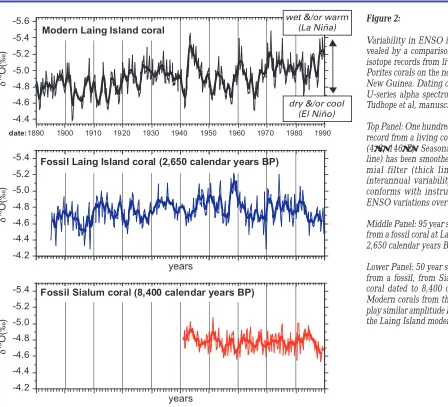
Figure 2 shows 3 oxygen isotope records from the north coast of Papua New Guinea: a modern record, a fossil coral dated at 2650 BP, and a fossil coral dated at 8400 BP (Tudhope et al., manuscript in prep.) This region of the far western equatorial Pacific experiences relative drought and lowered sea surface temperatures (SSTs) during the El Niño phase of the Southern Oscillation. These climatic factors are recorded in the oxygen isotopic composition of the skeletons of corals growing in nearby reefs, with isotopically heavy skeleton (less negative δ18O) deposited during the dry and cool El Niño events. Consequently, isotopic analysis of the annually banded skeletons of large living and ‘fossil’ mas-sive corals in the area can shed light on variations in the fre-quency and strength of ENSO.
Note the irregularity in all of these records. Strong and regular ENSO variability (~3–5 year periodicity) is evident from 1890 to 1925, and from the late 1960s until 1990, with a period of weak ENSO but large amplitude lower frequency variability in the intervening years (top panel). The 2,650 BP record (middle panel) shows modern-ENSO style variabil-ity (~3–5 year periodicvariabil-ity) in parts of the record, but much of the record is more like the weaker ENSO periods of the mid 20th century, and nowhere does the record show as
ex-treme a change as occurred in the early 1940s. Differences in the 8,400 BP record (Figure 2 bottom panel) are more clear-cut: there is variability in the typical 2–7 year ENSO band, but it is much weaker than in the other two records.
Pa-P
AGES/CLIV
AR Section
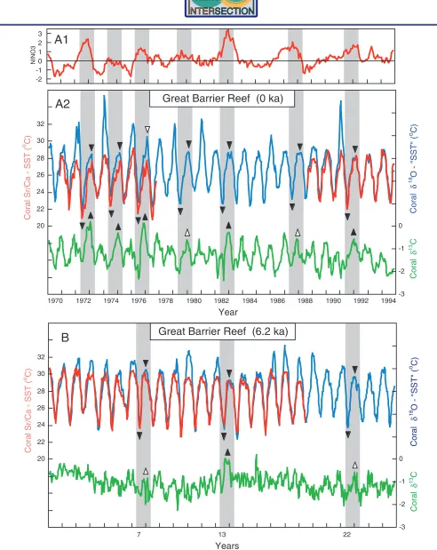
cific. Following the onset of El Niño, the 3-part sequence evident in the modern coral record includes: (i) relatively cool SSTs in the austral winter indicated by both the coral Sr/Ca and δ18O; (ii) reduced cloudiness in spring-summer indicated by the coral δ13C values; and (iii) lower than aver-age monsoon rainfall in summer shown by the δ18O. The strong El Niño events that are primarily confined to one an-nual cycle (1972/73, 1982/83, 1991/92) coincide with a strong 3-part signal in the coral record. At least 2 of the diagnostic indicators, usually cooler SSTs in winter followed by drought in summer, are observed during weak El Niños (1976/77, 1979/80, 1987/88).
Panel B in Figure 3 shows the same style of data for 6200 BP. In this 25 year long record, there is only one strong shift to El Niño. This event, in the middle of the record, clearly shows the 3 diagnostic features within the annual cycle that we know are associated with the development of an El Niño. The other 2 potential El Niños show winter SST cooling fol-lowed by drought, but the δ13C signal is weak. Perhaps they are weak events. The record is short, but taken at face value it shows weaker and less frequent ENSO activity at 6200 BP than at present. Note too, that SSTs were ~1°C warmer and rainfall less variable than in the modern period, reminiscent of a more La Niña like state in the mean.
The model behavior shown in Figure 1 is in rough agreement with the coral records in showing weaker ENSO activity in the mid-Holocene (6250 BP and 8400 BP) than in the modern. The ENSO cycle does continue, but strong events are less frequent (longer periodicity). The model ENSO vari-ability at 2650 is perhaps slightly stronger than in the mod-ern era, while the coral record (Figure 2) is slightly weaker. Given the high degree of variability within each record, it is hard to say whether this discrepancy is more than an arti-fact of limited sampling.
Thus the coral records generally support the model based the scenario given above. The model results demon-strate the possibility that the weakening of ENSO in the mid-Holocene results solely from orbitally forced changes in the tropical Pacific. Impacts of the extratropics or remnants of the glacial era are not needed, and could be no more than second order influences.
[image:5.595.35.483.66.473.2]The great variability within each of the sample records, coral or model, makes rigorous detailed comparison diffi-cult. Even with constant forcing the model generates decadal and longer timescale variability. This model is known to be a chaotic dynamical system (Tziperman et al., 1994). The same may well be true of the real system. Alternatively, the irregu-larity of the real ENSO may forced by atmospheric or oce-anic noise. The record is too short to determine which is the
Figure 2:
Variability in ENSO in the Holocene re-vealed by a comparison of stable oxygen isotope records from living and Holocene Porites corals on the north coast of Papua New Guinea. Dating of fossil corals is by U-series alpha spectrometry. Data from: Tudhope et al, manuscript in prep.
Top Panel: One hundred year skeletal δ18O
record from a living coral at Laing Island (4°S, 146°E). Seasonal δ18O data (thin
line) has been smoothed with a 9pt bino-mial filter (thick line) to help reveal interannual variability. This coral data conforms with instrumental records of ENSO variations over this period.
Middle Panel: 95 year skeletal δ18O record
from a fossil coral at Laing Island dated to 2,650 calendar years BP.
Lower Panel: 50 year skeletal δ18O record
P
AGES/CLIV
[image:6.595.54.546.39.658.2]AR Section
Figure 3:
A1: SST anomalies for the eastern equatorial Pacific (5°N–5°S, 90°W–150°W) as an indicator of the timing and magnitude of El Niño events (stippled bars; from Kaplan et al., 1998).
A2: Seasonal changes in Orpheus Island, central Great Barrier Reef (18°45’S, 146°29’E) coral Sr/Ca, δ18O, and δ13C. Stippled bars mark years
containing the 3-part sequence of environmental changes in the Great Barrier Reef that is diagnostic of El Niño: (1) cooler SSTs in the austral winter indicated by the coral Sr/Ca and δ18O; (2) reduced cloudiness in spring-summer indicated by higher coral δ13C values; and (3) reduced
monsoon rainfall in summer indicated by the coral δ18O. Black arrows indicate strong responses; weaker responses are indicated in white.
B: Sr/Ca, δ18O, and δ13C results for a mid-Holocene coral (TIMS 230Th age = 6,184 ± 34 yrs) from the same reef environment as the modern
calibration coral. The coral Sr/Ca and δ18O data were converted to temperature as defined by Gagan et al. (1998) and the δ18O data for the
P
AGES/CLIV
AR Section
Any definition of ‘abrupt‘ or ‘rapid‘ climate changes is nec-essarily subjective, since it depends in large measure on the sample interval used in a particular study and on the pat-tern of longer term variation within which the sudden shift is embedded. Here, we avoid any attempt at a general defi-nition but focus attention on different types of rapid transi-tion found in the paleo-record in different time periods of the geologically recent past. Although distinctions between types are somewhat arbitrary, together they cover a wide range of shifts in dominant climate mode on timescales rang-ing from the last half million years to the last few centuries.
1. Over the past half million years, marine, polar ice core
and terrestrial records all highlight the sudden and dramatic nature of glacial terminations, the shifts in global climate that occured as the world passed from dominantly glacial to inter-glacial conditions (e.g. Petit et al., 1999). These climate tran-sitions, although probably of relatively minor relevance to the prediction of potential future rapid climate change, do provide the most compelling evidence available in the his-torical record for the role of greenhouse gas, oceanic and biospheric feedbacks as nonlinear amplifiers in the climate system. It is such evidence for the dramatic effect of nonlinear feedbacks that, by very definition, supports the thesis that relatively minor changes in future climatic forcing may lead to dramatic, abrupt „surprises“ in climatic response.
2. Within glacial periods, and especially well documented
during the last one, spanning from around 110k to 11.6k years ago, there are dramatic climate oscillations, including high latitude temperature changes approaching the same magni-tude as the glacial cycle itself, recorded in archives from the polar ice caps, high to middle latitude marine sediments, lake sediments and continental loess sections. These oscilla-tions are usually referred to as Dansgaard-Oeschger Cycle and occur mostly on 1 to 2 kyr timescales (eg. Bender et al, 1999), although regional records of these transitions can show much more rapid change. The termination of the Younger Dryas cold event, for example, is manifested in ice core records from central Greenland as a near doubling of snow accumulation rate and a temperature shift of around 10oC
occurring within a decade (Figure 1, Alley et al., 1993). One hypothesis for explaining these climatic transitions is that the ocean thermohaline circulation flips between different stable modes, with warm intervals reflecting periods of strong deep water formation in the northern North Atlantic and vice versa (e.g. Stocker, 2000). It has been suggested that oscillation on this timescale is a persistent climatic feature which has continued throughout the Holocene, possibly in-cluding the Little Ice Age, albeit without the amplification associated with the presence of large Northern Hemisphere ice sheets (Bond et al., 1999). Should this prove to be the case, reason (Cane et al., 1995). Regardless of the cause, the high
degree of unforced variability makes it difficult to say with certainty that differences in the short coral records from dif-ferent periods are not just due to sampling fluctuations. A modern example of the same problem arises from a coral record reported at the workshop by J. Cole, which shows lower frequency behavior in the mid–19th century than at
present. The world was colder then; is there a causal rela-tionship? The discrepancies noted above between the model and coral data at 2650 BP could be significant, or could just be due to limited sampling. By the same token, the agree-ment at earlier times could be fortuitous. More rigorous sta-tistical analysis will sharpen the issue, and we plan to carry through such an analysis in the near future. However, it is most likely that this and similar issues can’t be settled with-out more coral records. Finding the right fossil corals is in good measure a matter of luck. Moreover, fossil coral records tend to be rather short, exacerbating problems of interpreta-tion. Another workshop talk, by C. Charles, illustrated a promising technique for overcoming this difficulty by join-ing series from different corals together, much as is done routinely for tree ring series. It appears realistic to believe that a coordinated program of modeling and fossil coral data acquisition could yield a reasonably complete picture of ENSO variations through the Holocene. Such a dataset would surely increase our understanding of ENSO dynamics, and our ability to tie ENSO variability to global changes through the Holocene.
References:
Cane, M. A., et al. Science, 275, 957–960, 1997.
Cane, M. A., et al. In Natural Climate Variability on Decadal-to-Cen-tury Time Scales, National Research Council, pp. 442–457, 1995. Clement, A. C., et al. Paleoceanography, 14, 441–456, 1999. Gagan, M., et al. Science, 279, 1014–1018, 1998.
Knutson, T. R., et al. J. Climate, 10, 131, 1997.
McGlone, M., et al. In El Niño. Historical and Paleoclimatic Aspects of the Southern Oscillation, (Diaz, H. & Margraf, V., eds.). Cambridge University Press, New York, pp. 435–462, 1992.
Meehl, G. & Washington, W. Nature, 382, 56–60, 1996. Rajagopalan, B., et al. J. Climate, 10, 2351–2357, 1997. Rodbell, D., et al. Science, 283, 516–520, 1999. Shulmeister, J. and Lees, B. Holocene, 5, 10–18, 1995. Timmermann, A., et al. Nature, 398, 694, 1999.
Trenberth, K. & Hoar, T. J. Geophys. Res. Lett., 10, 2221–2239, 1996. Tziperman, E., et al. J. Atmos. Sci., 52, 293–306, 1994.
Tziperman, E., et al., 1997: Mechanisms of seasonal-ENSO interac-tion. J. Atmos. Sci., 54, 61–71.
Wells, L. E. & Noller, J. S. Science, 276, 966–966, 1997.
Zebiak, S. E. & Cane, M. A. Mon. Wea. Rev., 115, 2262–2278, 1987.
Abrupt Climate Change
Keith Alverson and Frank Oldfield
PAGES IPO, Bern, Switzerland
P
AGES/CLIV
AR Section
the cycle would necessarily modulate higher frequency mate modes such as the NAO, and prediction of future cli-mate trends in the North Atlantic region would require ac-counting for these longer timescale processes.
3. During the first half of the Holocene, from 11.6k to around
6k years ago, evidence from lower latitudes especially points to rapid shifts in climate during the period when global ice volume, sea-level and vegetation were changing in the wake of the last glacial termination. Many of the changes taking place during the early Holocene, including melting of the polar ice caps, the rise of global sea level to something ap-proaching its present height, the recolonization of extensive areas by vegetation adapted to new climatic conditions and the maturation of soils resulting from increasingly stable vegetation cover, took millennia to complete. Thus, although it is tempting to use evidence of climate variability during the first half of the Holocene as an indication of possible ‘warm climate surprises‘, for all the reasons just noted, it is important to remember that the period was one of transi-tion. This said, it is equally important to dispel the view that the Holocene as a whole was a period of relatively constant climate. This proposition, arising from the stable isotope record in Central Greenland ice cores, is highly misleading. Not only is there now clear evidence of higher levels of cli-mate variability during the Holocene in Greenland itself, but at lower latitudes, evidence for Holocene climate variability is very strong.
One example of early Holocene rapid climate change is the ‘8200 BP’ cooling event recorded in the North Atlantic region (e.g. von Grafenstein et al., 1998). One possible expla-nation for this dramatic regional cooling is a shutdown in the formation of deep water in the northern North Atlantic due to fresh water input caused by catastrophic drainage of
Laurentide lakes (Barber et al., 1999). If this explanation proves to be correct it would lend support to the conjecture, based on numerical modeling experiments, that formation of deep water in the North Atlantic is highly sensitive to the fresh water forcing. This in turn would tend to reinforce the possibility of a rapid cooling ‘surprise’ in the North Atlantic region associated with potential future changes in the hy-drological cycle.
The whole of the early to mid-Holocene is marked by dramatic shifts in lake level and wetland extent in Africa and Central America. It is often difficult to gauge the pace of change from such records since many lakes in the region are, in part, the surface expression of ground water table varia-tions the response time of which is likely to be quite long. Nevertheless, in terms of the temporal resolution available and the expression of the hydrological changes in the archives studied, the major shifts appear to be rapid and of high am-plitude. Numerous modeling studies suggest that the abrupt-ness of the onset and termination of the early to mid-Holocene humid period across much of Africa north of the equator, depends on the presence of nonlinear feedbacks associated with both ocean circulation and changes in sur-face hydrology and vegetation (e.g. deMenocal et al., 2000). Without including these feedbacks alongside gradual inso-lation forcing, it is impossible for existing models to come even close to simulating the rapidity or the magnitude of climatic change associated with the extension of wetlands and plant cover in the Sahara/Sahel region prior to the on-set of desiccation around 5500 BP.
[image:8.595.38.296.66.269.2]4. For the last 6k years there are many more well dated high resolution records from a wide range of archives such as corals, tree rings and laminated lake sediments. There is also greater confidence in quantitative calibration through com-parison with instrumental records. Thus the concept of rapid change becomes something which can be better quantified though it is worth noting that our perception of particular changes will depend on the total time frame within which they can be set. Thus what appears as a sudden shift in mode of variability over a period of decades may be seen as a tran-sient event or part of an oscillating system on century or millennial timescales. The clearest examples of significant rapid shifts in climate during this period are most confidently discernible at regional scale or with respect to spatially con-strained modes of variability, for example, the major changes in frequency and strength of ENSO events noted by Cane et al, (this issue). When, as is the case with the changes associ-ated with the so-called Little Ice Age (LIA) and Medieval Warm Period (MWP), claims are made for at least hemi-spheric, if not global coherence, confirming widescale synchroneity becomes problematical (see Bradley, this issue). Many temporally well resolved proxy records show climate variability beyond the range revealed in modern in-strumental records from the same region. These records also include sudden shifts in mode. For example, Figure 2 shows a lake record from the central US which indicates a shift in the mode of hydrological variability occurred around 1200 AD, with the earlier portion of the record experiencing much more protracted and severe droughts than the later (Laird et al., 1996).
P
AGES/CLIV
AR Section
Although a thorough review is well beyond the scope of this note, these examples serve to highlight a wealth of evidence which exists for rapid climate changes during the Late Holocene; not always demonstrably globally or even hemispherically synchronous, but regionally highly signifi-cant. These changes are expressions of natural variability, the ongoing pattern of which will interact with and modu-late the expression of any anthropogenic climate change ef-fects. The underlying causes of the rapid changes now well documented remain uncertain in many cases. Some short term, extreme transient events clearly reflect the impact of major volcanic eruptions (Briffa,1998). In other examples, abrupt changes have been linked to 14C anomalies, a likely
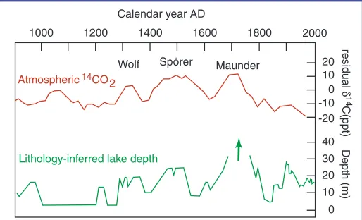
proxy for solar activity, as is the case with the widespread, major changes documented around 2650 BP by Van Geel et al. (1996) and the sequence of drought episodes reconstructed for Ethiopia by Verschuren et al. (2000) from lake sediment records covering the last 900 years (Figure 3).
5. The past 200 years span the period of major human envi-ronmental perturbation. Over this period greenhouse gas concentrations have risen extremely rapidly to levels that are unprecedented in at least the past 400,000 years (e.g. Raynaud, 2000). The magnitude and rate of measured glo-bal temperature rise during the past 200 years, on the other hand, does not appear to be unusual within the context of the Holocene. During the same 200 year period, the rate of land cover change has probably also been unprecedented in the Holocene. The apparent ENSO phase shifts during the 1970’s seems unique over this time period, and may thus represent a real climate shift (e.g. Trenberth and Hoar, 1997), although the available time series is probalby too short to unequivocally prove that the shift is significant (Wunsch, 1999). The inability to resolve questions of this kind from short instrumental time series provides one of the strongest arguments for extending the instrumental record of climate variability with well dated, temporally finely resolved and rigorously calibrated proxy data.
6. Implications for the future. Growing attention has been paid to the possibility of anthropogenic climate change lead-ing to ‘surprises‘ – shifts well beyond the range of variabil-ity upon which planning and construction schemes are based
and even outside the envelope of projections generated by climate models. The paleorecord does not preclude such possibilities.
One such potential ‘surprise’ that has been the target of several recent modeling studies is a shut down of North Atlantic Deep Water production occurring as an indirect re-sult of increasing greenhouse gas levels (Manabe and Stouffer, 1993) and possibly even in a manner sensitive to the rate of CO2 increase (Stocker and Schmittner, 1997). Re-gional climate changes linked to such an event would cer-tainly constitute a ‘surprise‘ and, for many parts of the world, possibly even a catastrophe.
Another example is the possibility of greenhouse gas driven warming leading to a change in the frequency of ENSO events. Modeling studies indicate that a strong en-hancement of ENSO conditions is not inconceivable (Timmerman et al., 1999). Such a drastic shift in ENSO fre-quency would have enormous consequences for both the biosphere and humans. Paradoxically, one possible conse-quence might be a sufficient increase in E-P forcing over the subtropical Atlantic to stabilize the thermohaline circulation (Schmittner et al., in press)
[image:9.595.24.381.73.235.2]The messages from the paleorecord for the future are not limited to these examples. Nor is belief in anthropogenic greenhouse gas warming an essential prerequisite for heed-Figure 2: Lake salinity record reconstructed for Moon Lake, North Dakota, illustrating regional drought variability over the last 2000 years. The severe droughts of the 1930’s and 1890’s (positive inferred salinity) are well reconstructed, but are eclipsed by more extensive droughts before the beginning of the instrumental period. There is an abrupt change in drought variability around AD 1200. Before that time, the high plains were characterized by much more regular and persistent (e.g., interdecadal) droughts. The mechanisms for major shifts in drought variability of the past are not well understood, and no processes model has successfully simulated these types of changes. Note that the gap in 17th century data coverage represents absence of data. (Source: Laird et al., 1996)
[image:9.595.301.558.584.740.2]P
AGES/CLIV
AR Section
Improving Estimates of Drought Variability and Extremes from Centuries-Long Tree-Ring Chronologies: A PAGES/CLIVAR Example
Edward R. Cook, Mike Evans
Lamont-Doherty Earth Observatory, Palisades, NY 10964 [email protected]
The impact of severe drought on agriculture, water supply, and the overall environment is an increasing global concern as the demand for water outstrips supplies in many areas of the world. Reliable long-range forecasting methods need to be developed to allow agricultural and water resource plan-ners and administrators to reduce the impact of future droughts. In addition, longer climate records are needed for improving regional drought risk assessments, especially those dealing with the rare, extreme events. For both pur-poses, the instrumental climate database is likely to be inad-equate, even in the well monitored U.S. It is very difficult to know if the instrumental records are long enough to include the full range of drought variability likely to happen in any given region in the future. This issue was specifically ad-dressed in a recent workshop convened by NOAA and NASA: “Assessing the Full Range of Central North America Droughts and Associated Landcover Change”, Boulder, Colorado, June 2–4, 1999. One conclusion drawn from this workshop was that instrumental climate data over the U.S. are inadequate for capturing the “full range” of drought. Consequently, there is an urgent need to develop long records of past drought from a variety of proxy records. Among those available, precisely dated annual tree-ring chronologies from centuries-old trees growing on drought-stress sites are ide-ally suited for this pupose.
A recent paper by Woodhouse and Overpeck (1998) has likewise highlighted the limitations of instrumental cli-mate data by examining the paleoclicli-mate record of drought in the western U.S. They find evidence of past “megadroughts” of unusual severity and duration in the paleoclimatic record, ones that appear to have exceeded even the Midwestern “Dustbowl” drought of the 1930s. The analy-sis of Woodhouse and Overpeck (1998) illustrates the tre-mendous value of paleoclimate data in studying past drought. However, it also shows the current limitations of the available proxy records. Among the data they use is the 154 grid point network of well-calibrated and verified sum-mer drought reconstructions from annual tree-ring chronolo-gies produced by Cook et al. (1999) for the coterminous U.S. This network, based on the Palmer Drought Severity Index (PDSI; Palmer, 1965), provides a highly detailed record of drought and wetness over the U.S. in both space and time. Unfortunately, these reconstructions only extend back to 1700 at the present time. Yet, Woodhouse and Overpeck (1998) clearly show in a sparser collection of much longer individual drought reconstructions that some notable megadroughts occurred in the western US, mostly prior to AD 1600. There-fore, there is a great need to produce a substantially longer, high-density network of drought reconstructions for the U.S. that extends 600–800 years back into the past. Such a net-work would provide the means to carefully map the occur-rence of drought during these megadrought periods. In so ing these messages. Extending the record of climate
vari-ability back through time reveals changes, often sudden and sometimes persistent on decadal to century timescales that lie outside the range of instrumental records. The concepts of future sustainability, water supply and food security may be dangerously short sighted if they fail to accommodate the evidence from the longer term record. This is especially the case in relation to changes in the magnitude and fre-quency of extreme events (e.g. Knox, 2000) and to shifts in hydrological regime (e.g. Hodell et al., 1995; Messerli et al., 2000). The growing consensus however, is that future cli-mate change will reflect not only natural variability but an-thropogenic forcing as well. It is interesting to compare even the most modest predictions of greenhouse warming with natural variability recorded in the recent past. Even though the last six centuries appear to have recorded both the coldest and warmest decades to have occurred in the late Holocene (e.g. Bradley, 2000), the amplitude of variation in Northern Hemisphere mean annual temperature between these ex-tremes is less than the lowest projected temperature increases for the next century.
References:
Alley, R., et al. Nature, 362, 527–229, 1993. Barber, D., et al. Nature, 400, 344–348, 1999.
Bender, M., et al. In: Mechanisms of Global Climate Change, (P. Clark et al. eds). AGU, 149–164, 1999.
Bond, G., et al. In: Mechanisms of Global Climate Change, (P. Clark et al. eds). AGU, 35–58, 1999.
Bradley, R. (this issue)
Bradley, R. In: Past Global Changes and Their Significance for the Fu-ture, (K. Alverson et al. eds.). Quaternary Science Reviews, 19, 1–5, 391–402, 2000.
Briffa, K., et al. Nature, 393, 450 – 455,1998. Cane, M., et al. (this issue)
DeMenocal, et al. In: Past Global Changes and Their Significance for the Future. (K. Alverson et al. eds.). Quaternary Science Reviews, 19, 1–5, 347–361, 2000.
Hodell, D.A., et al.Nature, 375, 391 – 394, 1995.
Knox, J.C. In: Past Global Changes and Their Significance for the Fu-ture, (K. Alverson et al. eds). Quaternary Science Reviews, 19, 1–5, 439 – 458, 2000.
Laird, et al. Nature, 384, 552–554, 1996.
Messerli, B., et al. In: Past Global Changes and Their Significance for the Future, (K. Alverson et al. eds). Quaternary Science Reviews, 19, 1–5, 459 – 479, 2000.
Petit, et al. Nature, 399, 429–436, 1999.
Raynaud, D., et al. In: Past Global Changes and Their Significance for the Future, K. Alverson et al. eds. Quaternary Science Reviews, 19, 1– 5, 9–18, 2000.
Schmittner, et al. Geophys. Res. Lett., in press.
Stocker, T. In: Past Global Changes and Their Significance for the Fu-ture, (K. Alverson et al. eds). Quaternary Science Reviews, 19, 1–5, 301–319, 2000.
Stocker, T. & A. Schmitttner Nature, 388, 862–865, 1997. Timmermann, A., et al. Nature, 398, 694–696, 1999.
Trenberth, K. & T.J. Hoar. Geophys. Res. Lett., 24, 3057–3060, 1997. Van Geel, B., et al. J. Quaternary Science, 11, 275 – 290, 1996. Verschuren, et al. Nature, 403, 410–414, 2000.
P
AGES/CLIV
AR Section
doing, it may be possible to analyze the spatial patterns and evolutive trajectories of these megadroughts and infer their causes.
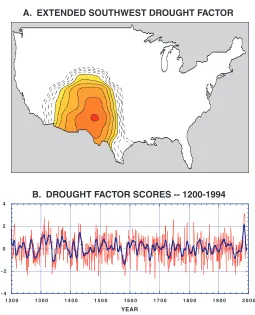
To illustrate the importance of extending the drought reconstructions further back in time, we have applied opti-mal interpolation (OI; Kaplan et al., 2000) to the U.S. PDSI reconstruction grid (Cook et al., 1999) after it had been aug-mented with a number of much longer tree-ring estimates in certain parts of the network. This has enabled us to use OI to extend the PDSI reconstructions over the entire U.S. from 1200 to 1994. Figure 1 shows the first varimax rotated EOF of reconstructed PDSI and its scores using the extended OI PDSI data. This factor emphasizes the southwestern US and is probably the highest quality region produced by the OI analysis. The OI scores have a correlation of 0.77 with in-strumental PDSI from the Southwest on an annual basis and 0.86 on a smoothed, inter-decadal basis over the period 1895–1994. They also have a correlation of 0.93 with the varimax factor scores for the same region based on non-in-terpolated PDSI reconstructions over the common period 1469–1978.
The factor scores clearly illustrate the importance of extending the drought reconstructions as far back in time as possible. Prior to 1600, there is evidence for three megadroughts in the 1280s, 1340s, and 1580s. The 1280s “Great Drought” has been associated with the disappear-ance of the Anasazi indian culture in the Southwest (Douglass 1929); and the 1580s drought is coincidental (perhaps linked) with the drought associated with the disappearance of the colonists on Roanoke Island (Stahle et al. 1998). Woodhouse and Overpeck (1998) also document the occurrence of the 1280s and 1580s droughts in the western US, but do not de-scribe the 1340s event indicated here. Besides having three of the worst droughts of the past 800 years, the AD 1200– 1600 interval is also characterized by enhanced inter-decadal variability that is associated with more prolonged episodes of drought and wetness. This is clearly illustrated in the fol-lowing table, which lists the five driest 5, 10, and 20-year periods in this southwestern US drought record.
5-Year Period 10-Year Period 20-Year Period Rank Dates Mean Dates Mean Dates Mean
[image:11.595.304.559.60.375.2]1 1581–1585 –1.717 1576–1585 –1.442 1573–1592 –1.008 2 1666–1670 –1.584 1338–1347 –1.237 1336–1355 –0.730 3 1338–1342 –1.479 1664–1673 –1.010 1273–1292 –0.709 4 1399–1403 –1.343 1728–1737 –0.987 1945–1964 –0.629 5 1421–1425 –1.289 1280–1289 –0.910 1445–1464 –0.609
Table 1. List of the five driest 5, 10, and 20-year periods in the PDSI factor scores shown in Fig. 1. The units are in standard normal deviates. Note the prevalence of megadroughts in the AD 1200–1600 pe-riod that would be totally missed if the PDSI reconstructions only extend back to, say, 1600.
Note that for both the 5-year and 20-year intervals, 4 of the 5 driest periods were in the AD 1200–1600 epoch. Also, the late–16th century drought examined by Stahle et al.
(2000) appears to be the megadrought of the past 800 years in the southwestern US. Thus, it is clear that PDSI recon-structions covering only the past 300–400 years are not suffi-cient to capture the full range of drought/wetness
variabil-ity across the coterminous US. In fact, the recent few centu-ries could be interpreted as being conspicuously deficient of megadroughts, due perhaps to climate associated with the “Little Ice Age” (see Bradley, this issue). Why this is so is a mystery that needs to be solved and modeled. Any return to the modes of climate variability characteristic of the pre–16th
century period in the US Southwest would be diasterous. If we truly want precisely dated, annual estimates of past drought for improving our understanding of drought vari-ability and extremes, and for testing hypothesized forcings of drought and wetness (e.g. Cole and Cook, 1998; Cook et al., 1997), the only recourse is to use centuries-long tree-ring chronologies and novel statistical estimation procedures to reconstruct the past.
References
Cole, J.E. & E.R. Cook Geophys. Res. Lett., 25, 4529–4532, 1998. Cook, E.R., et al. J. Climate, 10, 1343–1356, 1997.
Cook, E.R., et al. J. Climate, 12, 1145–1162, 1999.
Douglass, A.E. National Geographic Magazine, 56, 736–770, 1929. Kaplan, A., et al. J. Climate, in press.
Palmer, W.C., 1965: Meteorological Drought. Research Paper No. 45, U.S. Dept. of Commerce Weather Bureau, Washington, D.C.
Figure 1:
(A) The first varimax rotated Empirical Orthogonal Function (EOF) of a Palmer Drought Severity Index (PDSI) grid derived from optimally interpolated tree ring chronologies. This factor emphasizes the south-western US and is probably the highest quality region produced by the analysis.
P
AGES/CLIV
AR Section
Stahle, D.W., et al. Science, 280, 564–567, 1998.
Stahle, D.W., et al. EOS, Transactions of the American Geophysical Union, in press.
Woodhouse, C. & J.T. Overpeck. Bull. Amer. Meteoro. Soc., 79, 2693– 2714, 1998.
Conceptual Framework for Changes of Rainfall and Extremes of the Hydrological Cycle with Climate Change
Kevin E. Trenberth
National Center for Atmospheric Research1, Boulder, USA
1The National Center for Atmospheric Research is sponsored by the National Science Foundation.
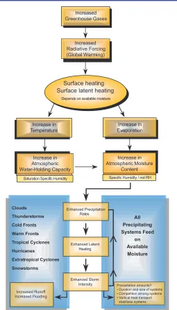
A physically based conceptual framework is put forward that explains why an increase in heavy precipitation events should be a primary manifestation of the climate change that accompanies increases in greenhouse gases in the atmos-phere. The same arguments apply generally for all kinds of climate change. This paper summarizes Trenberth (1998, 1999) and a full set of references is given in those works.
The term “global warming” is often taken to refer to global increases in temperature accompanying the increases in greenhouse gases in the atmosphere. In fact it should re-fer to the additional global heating (sometimes rere-ferred to as radiative forcing, e.g., by the IPCC (1996)) arising from the increased concentrations of greenhouse gases, such as carbon dioxide, in the atmosphere. Increases in greenhouse gases in the atmosphere produce global warming through an increase in downwelling infrared radiation, and thus not only increase surface temperatures but also enhance the hy-drological cycle, as much of the heating at the surface goes into evaporating surface moisture. This occurs in all climate models regardless of feedbacks, although the magnitude varies substantially.
Temperature increases signify that the water-holding capacity of the atmosphere increases and, together with en-hanced evaporation, the actual atmospheric moisture should increase, as is observed to be happening in many places. Of course, enhanced evaporation depends upon the availabil-ity of sufficient surface moisture and over land, this depends on the existing climate. However, it follows that naturally-occurring droughts are likely to be exacerbated by enhanced potential evapotranspiration. Further, globally there must be an increase in precipitation to balance the enhanced evapo-ration but the processes by which precipitation is altered lo-cally are not well understood.
Precipitating systems of all kinds feed mostly on the moisture already in the atmosphere at the time the system develops, and precipitation occurs through convergence of available moisture on the scale of the system. Hence, the at-mospheric moisture content directly affects rainfall and snowfall rates, but not so clearly the precipitation frequency and thus total precipitation, at least locally. Thus, it is ar-gued that global warming leads to increased moisture con-tent of the atmosphere which in turn favours stronger rain-fall events, as is observed to be happening in many parts of
the world, thus increasing risk of flooding. It is further ar-gued that one reason why increases in rainfall should be spotty is because of mismatches in the rates of rainfall ver-sus evaporation.
The arguments on how climate change can influence moisture content of the atmosphere, and its sources and sinks are assembled in the schematic in Fig.1. The sequence given is simplified by omitting some of the feedbacks that can in-terfere. For example, an increase in atmospheric moisture may lead to increased relative humidity and increased clouds, which could cut down on solar radiation (enhance short-wave cloud forcing) and reduce the energy available at the surface for evaporation. Those feedbacks are included in the climate models and alter the magnitude of the surface heat available for evaporation in different models but not its sign. Figure 1 provides the rationale for why rainfall rates and frequencies as well as accumulations are important in understanding what is going on with precipitation locally. The accumulations depend greatly on the frequency, size and duration of individual storms, as well as the rate and these depend on static stability and other factors as well. In par-ticular, the need to vertically transport heat absorbed at the surface is a factor in convection and baroclinic instability both of which act to stabilize the atmosphere. Increased green-house gases also stabilize the atmosphere. Those are addi-tional considerations in interpreting model responses to in-creased greenhouse gas simulations.
However, because of constraints in the surface energy budget, there are also implications for the frequency and/or efficiency of precipitation. The global increase in evapora-tion is determined by the increase in surface heating and this controls the global increase in precipitation. But precipi-tation rates are apt to increase more rapidly, implying that the frequency of precipitation must decrease, raising the possibility of fewer but more intense events.
It has been argued that increased moisture content of the atmosphere favours stronger rainfall and snowfall events, thus increasing risk of flooding. Although there is a pattern of heavier rainfalls observed in many parts of the world where the analysis has been done, flooding records are con-founded by changes in land use, construction of culverts, dams and so forth designed to control flooding, and increas-ing settlement of flood plains which changes vulnerability to flooding.
P
AGES/CLIV
AR Section
events, yet still deal with whole storms rather than individual rain cells, hourly precipitation data are recommended. Such data are also retrievable from climate models.
References
IPCC: Climate Change 1995. Eds. J. T. Houghton, et al., Cambridge Univ. Press, Cambridge, U.K., 572pp, 1996.
[image:13.595.26.281.67.514.2]Trenberth, K. E. Climatic Change, 39, 667–694, 1998. Trenberth, K. E. Climatic Change, 42, 327–339, 1999.
Figure 1: Schematic outline of the sequence of processes involved in cli-mate change and how they alter moisture content of the atmosphere, evaporation, and precipitation rates. All precipitating systems feed on the available moisture leading to increases in precipitation rates and feedbacks. (Trenberth, 1998)
Century to Decadal Scale Records of Norwegian Sea Surface Temperature Variations of the past 2 Millennia
Eystein Jansen
Dept. of Geology, Univ. of Bergen, Bergen, Norway [email protected]
Nalan Koç
Norwegian Polar Institute, Tromsø, Norway [email protected]
Recent focus on rapid climate change and millennial scale climate variability in paleoceanography has led to a marked improvement in the temporal resolution of paleoceanographic climate records. Recent studies have in-dicated a possible existence of pervasive cycles of oceanic variability at approximately 1500 years, both in surface wa-ters and in the strength of North Atlantic deep water flows (Bond et al., 1997; Bianchi and McCave, 1999). These cycles appear to continue into the Holocene (postglacial phase – i.e. the last 11,000 years). The last such event may have been the warm-cold alteration normally associated with the Me-dieval Warm Period (MWP) centred at approximately 1000 AD, and the Little Ice Age (LIA) between 1400 and 1800 AD in Europe. This increased potential for detailed paleoclimatic records from rapidly accumulating sediments, as docu-mented by these and other results, has spurred much inter-est in the community. The focus has been on obtaining ultra high temporal resolution from sediment cores retrieved from areas where sediment focusing expands the sections and enables detailed sampling. It is also a prerequisite that it is possible to utilise the normal methods of paleoclimatic esti-mation. This would require open ocean settings and a tem-poral resolution approaching decadal scale in the best cases. In some very restricted areas annually laminated sediments may be found, which may provide annually resolved paleoclimate records. Outside of these areas, one would need to obtain cores from rapidly deposited sediments in areas of high sediment focusing. Annual resolution is not feasible here.
Using this approach, a pilot study was conducted in high accumulation rate sediments from the Vøring Plateau in the Eastern Norwegian Sea at 67oN (IMAGES core MD95–
2011). The study documents SST-variations during the last millennia at hitherto unprecedented resolution (Fig. 1b) from this kind of research. This indicates that careful selection of cores will enable quantitative estimates of ocean proxies ap-proaching decadal scale (see below). The core is dated by
210Pb and AMS-14C (6 dates for the past 2000 years). We
esti-mate the accuracy of the time scale to be about 50 years, which may be somewhat improved in the future by more detailed AMS 14C-chronology. The summer SST is estimated using
diatom transfer functions. Parallel work using other SST-es-timation techniques are underway.
influ-P
AGES/CLIV
AR Section
ence of declining summer insolation by the orbital factors. Both the MWP and a two-phased LIA are detectable in the data set, as well as rapid cooling and warming intervals, happening over a decade: Note cold-warm-cold phase in the period 1300–1450 AD according to the time scale of the core. Possible century scale cycles may be identified in the data set, but await improved chronological control.
In the figure we have compared this record with the SST record from Bermuda Rise over the same time period recently published (Keigwin, 1996; Keigwin and Pickart, 1999) (Fig. 1A). The lower temporal resolution of the sedi-ment section and possibly a higher degree of bioturbation at this site, has probably worked as a low pass filter on the variability over Bermuda Rise. Hence, only the main multi-centennial scale variations may be compared at this stage. SST changes associated with the MWP and LIA at Bermuda Rise were of the same order of magnitude as in the Norwe-gian Sea. The timing of the warm and cold phases are not identical. This may be due to the bioturbation filtering, time scale problems, or time scale inaccuracies. Hence, improved temporal resolution and chronologies are required to fur-ther compare the spatial SST variability in the North Atlan-tic. An important path to follow by further investigations is the intriguing proposition of Keigwin and Pickart (1999). They suggest that opposite SST anomalies between the West-ern North Atlantic and the Labrador Sea region were devel-oped during the LIA in a similar way as the anomaly pat-tern known from the NAO phases (see Sarachik, this issue). This work is now underway. Under the auspices of the PAGES marine program, IMAGES, a large community based coring expedition was conducted in the summer of 1999, using the unique large coring system of the French RV Marion Dufresne. A large number of sites dedicated for ultra-high resolution studies of this type were cored in the Circum Atlantic and the Nordic Seas. A new era of very high-resolu-tion paleoceanographic reconstruchigh-resolu-tions has been initiated by this cruise, and a wealth of new high quality data can be expected in the next years. This holds good promise for fu-ture interaction between the paleoceanogrphy community of PAGES and CLIVAR.
Acknowledgements: We acknowledge support from the EU-Environment and Climate Programme, the Norwegian Re-search Council and the French CNRS/IFRTP for supporting the IMAGES coring expeditions.
References
Bianchi, G.G. & I.N. McCave. Nature, 397, 515–517, 1999. Bond, G., et al. Science, 278, 1257–1266, 1997.
Keigwin, L.D. Science, 274, 1504–1508, 1996.
Keigwin, L.D. & R.S. Pickart. Science, 286, 520–523, 199?.
Opportunities for CLIVAR/PAGES NAO Studies
E.S. Sarachik
University of Washington, Seattle, USA [email protected]
K. Alverson
PAGES IPO, Bern, Switzerland [email protected]
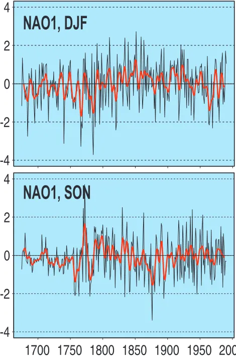
[image:14.595.313.559.69.387.2]The normal atmospheric situation over the North Atlantic Ocean has surface westerlies blowing across the ocean at about 40°N between the surface expression of the Icelandic low and the Azores high, with the most intense westerlies existing during the winter season. On times scales ranging from monthly to interdecadally, there is an oscillation of the strength of these pressure features which can be conveniently measured by the difference in surface pressure between the Azores (or some nearby station) and Iceland. The state of this North Atlantic Oscillation (NAO) is positive when the Azores high is strong and the Icelandic low is deep and nega-tive when reversed. A time series of this normalized winter index is given in Fig. 1.
P
AGES/CLIV
[image:15.595.296.558.62.491.2]AR Section
Figure 1: Updated winter NAO index based on instrumental data. Courtesy of P.D. Jones to T. Osborn (http://www.cru.uea.ac.uk/~timo/ projpages/nao_update.htm)
The extraordinary climatic interest in the NAO arises from two observations: the unusual locking of the NAO in its positive phase almost continuously since 1976 and the concomitant collection of climatic phenomenon which can be associated with its positive and negative phases. These two phases are given by the two parts of Figure 2.
The Positive phase of the NAO is mostly easily char-acterized during the winter and has the following effects:
•
Stronger Westerlies across the Atlantic extending further north towards the British Isles and pointing toward northern Europe;•
A more intense storm track roughly steered by the dis-placed westerlies;•
Stronger upwelling off the coast of Portugal and North-western Africa due to the southerlies accompanying the intensified Azores high;•
Stronger (easterly) trades off the coast of Africa into the subtropical Atlantic;•
Wet anomalies over the eastern US coast extending across the Atlantic into Scandinavia and northern Siberia;•
Dry anomalies over the Labrador sea and over South-ern Europe and the Mediterranean region;•
Wet anomalies over northern Africa extending eastward into the Arabian Sea;•
Warm anomalies over major parts of the US (as far west as Alaska), northern Europe and extending eastward all the way across Siberia;•
Cold anomalies over the Labrador Sea and simultane-ous warm anomalies over the GIN seas;•
Increased ice flux out of the Artic Ocean from the Fram Straits.There are also direct effects of NAO variability on the ocean, both in terms of direct driving of fluxes by the NAO (Cayan, 1992) and in convective responses to NAO changes in heat and freshwater inputs (Dickson et al., 1996).
We may note that the Pacific manifestations of the NAO are consistent with the idea that the NAO itself is part of a more annular (circumpolar) mode of variability that has expression in both the North Atlantic and Pacific (Thompson
and Wallace, 1998). For the purposes here, we will not dis-tinguish between the NAO and the so-called Arctic Oscilla-tion (AO). We might also note that the above menOscilla-tioned positive phase of NAO since 1976 is coincident with (and may be related to), the rapid global surface warming, espe-cially at high latitudes, evident in the record.
Paleoclimatic Opportunities:
[image:15.595.25.282.87.213.2]P
AGES/CLIV
AR Section
before. Therefore, in order to better interpret the instrumen-tal record of NAO variability it is imperative that a longer record be obtained.
Several paleoclimatic proxies have the potential to record aspects of North Atlantic climatic variability, and thereby the NAO index, with annual or higher resolution to well before the year 1700. Recent paleo-proxy NAO recon-structions with annual or better resolution include, for ex-ample, those from tree rings (Cook et al., 1998), ice cores (Appenzeller et al., 1998), stalagmites (Proctor et al., in press) as well as combined tree ring and ice core data (Stockton and Glueck, 1999). Regional synthesis of paleo-proxy indi-cators with subdecadal resolution can provide information regarding historical impacts of the NAO on regional mois-ture balance. One example is the multiproxy regional syn-thesis of historical records, tree-rings, laminated lake sediments, speleothems, geomorphological and other sources in the Mediterranean region currently being under-taken as part of the PAGES PEP III synthesis (detailed infor-mation on this program will be published in the upcoming PAGES Newsletter Vol.8, N°2). Multiple proxies in the Scandinavian region, including annually laminated lake sediments, tree rings, glaciers and speleothems provide an-other fruitful area for future paleoclimatic synthesis of NAO variability and regional expression in the past.
Luterbacher et al. (1999) have published a multiproxy derived NAO index with monthly resolution from 1675 to the present. Their reconstruction is shown in figure 3. In addition to the reconstruction, Luterbacher et al.show that the correlations between the many individual paleo recon-structions that are now available are not high enough to re-gard any one of them as definitive. An approach which in-cludes multiple, independent, paleoclimatic archives and proxies is clearly required in order to provide an extended record of NAO variability. Such studies are underway (e.g. Cullen et al., submitted) and will lead, in the next few years, to both an improved record of NAO variability as well as better understand the underlying dynamics associated with this important mode of climatic variability.
References:
Appenzeller, C., et al. Science, 282, 446–449, 1998. Cayan, D. J. Climate, 5, 354–369, 1992.
Cook, E.R., et al. Holocene, 8, 9–17, 1998.
Cullen, H.M, et al. (preprint available from http:// rainbow.ldeo.columbia.edu/climategroup/papers/paleo_finaltimes.pdf), submitted to Paleoceanography
Dickson, R., et al. Oceanography, 38, 241–295, 1996. Luterbacher, J., et al. Geophys. Res. Lett., 26, 2745, 1999.
Stockton, C.W. & M.F. Glueck Proceedings of the Amer. Meteor. Soc. 10th Symposium on Global Change Studies, 290–293, 1999.
Thompson, D.W. & J.M. Wallace. Geophys. Res. Lett., 25, 1297–1300, 1998.
[image:16.595.47.282.70.424.2]Wunsch, C. Bull. Amer. Meteor. Soc., 80, 245–255, 1999.
P
AGES Section
PAGES Section
Reconstructing Climatic Variability from Historical Sources and Other Proxy Records
Henry F. Diaz
Climate Diagnostics Center, NOAA, Boulder, USA [email protected]
An international conference titled, “Reconstructing Climatic Variability from Historical Sources and Other Proxy Records” was held in Manzanillo, Mexico, on 1–3 December, 1999. The meeting attracted 21 participants from 9 countries. The goal of the conference was to highlight historical research directed at reconstructing climatic variations prior to the modern era of instrumental records. A special focus was on historical climate research in the Americas, although a number of pa-pers also focused on new results from other parts of the globe. In addition, some papers specifically addressed this topic from the perspective of epidemiological history and the pos-sible role that climatic variations may have had in initiating and/or exacerbating communicable diseases, especially vec-tor borne illnesses.
Papers were presented covering three major themes: 1) Reconstructing major drought and flood episodes, prima-rily in the region of the Americas for the past four centuries; 2) Documenting multiscale teleconnections and their asso-ciation with El Niño/Southern Oscillation (ENSO) events and other decadal climate variability, such as the North At-lantic Oscillation (NAO); and 3) Emerging studies on the con-nections between climate and human health. A central goal of the meeting was to advance the study of historical analy-sis for the purposes of emphasizing those times where sig-nificant historical events and periods may have been affected by major climatic events—prolonged cold episodes or ex-tended drought, perhaps associated with the occurrence of extreme events such as ENSO, or large volcanic eruptions. Another goal of the conference was to promote the exchange of views and information among the participants, and to foster new ideas for collaborative research.
The papers presented at the conference underscore the wide depth and breadth of ongoing research, and illustrate the potential of this type of analysis within the study of long term climate change. There exists in the Americas, as well as in many other parts of the world, rich sources of archived information that can be used to infer climatic changes in the past, on annual, interannual, and decadal timescales. Below, a few of the more promising studies and their possible use in climatic reconstruction are highlighted.
In the United States, large amounts of weather and climate information were recorded, mostly in diaries during the 19th century by pioneers moving west across the
conti-nent, primarily from the 1840s onward. In the earlier-settled eastern United States, useful climate information can be ex-tracted from diaries and other such documentary records back to the start of the 19th century, and earlier in a few
in-stances. The beginnings of organized weather and climate services in other parts of the Americas generally parallel those in the U.S. and Europe, because many of the major figures that played important roles in that development were from Europe or the U.S.A. High-resolution climate proxies can be extracted in places where the daily state of the weather was important for commercial reasons. For instance, high mountain passes in the Andes of South America, which were an important transportation artery between major settle-ments, recorded daily snow conditions for much of the year. Normalized time series of snowfall quantity have been de-veloped from the mid–1700s for an area in the central Andes along the Argentinean–Chilean border.
Other presentations focused on continuing efforts to improve and refine the chronology of El Niño events prior to the modern instrumental records, which go back to about the mid–1800s. These efforts include the mining of informa-tion about weather phenomena usually associated with ENSO events from a variety of sources, as well as the use of coral records from the tropical Pacific. New information use-ful for the analysis of long term variations in the NAO has been developed from the Canary Islands, using agricultural time series as proxies for precipitation. Another interesting set of proxy records is the voyage durations of the Manila Galleons, whose yearly trips from Acapulco, Mexico to Ma-nila, The Phillippines, starting in the late 1500s, and continu-ing for more than two centuries, may be able to provide a record of decadal scale variability in the strength of the North Pacific trade winds. The utility of comparative analysis among different proxy records was illustrated by the fact that a period of apparently weaker trades in the western tropical Pacific, inferred from the presence of significantly longer voyage durations of the Manila Galleons from about 1630–1680, coincides with a large increase in the incidence of typhoon landfalls in sou


![Figure 1: (A) SST-summer estimates for the last 2000 years at Ber-muda Rise. From [Keigwin and Pickart, 1999]](https://thumb-us.123doks.com/thumbv2/123dok_us/1038545.619379/14.595.313.559.69.387/figure-sst-summer-estimates-years-rise-keigwin-pickart.webp)