Abstract—An analysis aiming the common roots of polynomial equations, their multiple roots and elimination of certain variables, have been carried out, completing questions not found in the known literature. Certain improvements concern the construction of a diagram for a matrix method. Another interesting analysis concerns the procedures for applying direct methods. It resulted that even if the computations differ, the results do not differ. The symbolic language led to a high facility of the analysis.
Keywords—Theory of equations, common multiple roots, elimination, symbolic language.
I. INTRODUCTION
In order to make an analysis as clear as possible, and useful for practical applications, several approaches have to be examined, among which: the elimination of one or more variables, between two or more equations, respectively, the search of common roots (of a set of equations) or of multiple roots (of one equation), and then, the use of Maple 12 software.
The elimination has been frequently used in many applications. We shall mention the meaning of this operation in the known literature.
To eliminate some terms from a system of equations, means to express one or more variables from that system of equations in terms of the quantities existing in certain equations, and to introduce them into other equations of the considered system, so that, these variables of the system vanish.
In this manner, starting from a system of n
equations, one can derive another system of the same number or a smaller number of equations, in which, certain variables do not occur any more.
Many studies have been carried out in this domain or related to it [1]-[9], however certain problems not examined in the known literature are analyzed in the present paper. For the sake of clarity, we chose to make the explanations using certain examples, one concerning the Sylvester method, another concerning
Manuscript received 23rd November, 2013. Professor Andrei
Nicolaide is with the “Transilvania” University of Brasov, Romania. Address: “Transilvania” University of Brasov, Bd. Eroilor Nr. 29, Brasov, Cod 500036, Romania (e-mail: [email protected]).
the method of direct calculation, and finally only Maple 12 software.
II. THE PROGRESS IN THE FIELD
It is worth noting to mention that J. L. Lagrange (in 1770) has examined the conditions for two algebraic equations have just p common roots.
Several geometers: G. W. Leibniz (1646-1716), L. Euler (1707-1783), E. Bézout (research around 1756), H. G. Zeuthen (1839-1920), J. G. Darboux (1842-1917), (in 1876), J. J. Sylvester (1814-1897), Eugène Rouché (1832-1910), (in 1877), made important progress in this field, minutely analyzed by Ch. Comberousse (1826-1897), [3], and Eberhard Knobloch [1].
The calculations for eliminating an unknown between two equations and keeping a single one, and those for the two equations have a common root, are similar, but not completely, as further shown. For examining the matrix method, of Sylvester, actual denomination, at the time, more used, determinant and table, let us consider two algebraic equations.
For practical applications, several approaches have to be examined, among which: the elimination of one or more variables, between two or more equations, and the search of common roots (of a set of equations) or of multiple roots (of one equation).
III. THE SYLVESTER METHOD
Despite the numerous studies in this domain or related to it, [1]-[9], there are certain problems not solved in the known literature. For to fix the ideas. We shall make the explanations on certain examples concerning the Sylvester method. For this purpose, let us consider the two algebraic equations below:
( )
x ax i[
m]
F = i m−i,∀ ∈ 0, , (1 a)
( )
x ax i[ ]
nf = i n−i,∀ ∈0, , (1 b)
of degrees m and n . We have proposed some simplification, for the construction of the matrix, as well as, for the involved calculations. For solving such a system, it is possible to convert this system of two equations into a single system, each term of it maintaining its coefficient but being brought at the same exponent on the same column. For this purpose,
An Approach to Common Roots and
Elimination of Variables by Using a Symbolic
Programming Language
both sides of equation (1 a) will be successively multiplied, with each term of the (n−1) terms of the sequence xn−j,∀j∈
[ ]
1, n , n being the degree of equation (1 b). Therefore, for the first row (line), the exponents will decrease from m+n−1 to m. Then, both sides of equation (1 b), will be successively multiplied, with each of the (m−1) terms of the sequence xm−j,∀j∈[
1, m]
, m being the degree of equation (1 a).Similar calculations are carried out for both, equations (1 a) and (1 b).
The obtained equations may be considered as a system of m+n linear equations, each unknown being of the form xm+n−1. According to the present form of the procedure along every row, the index
(
n−i)
and(
m− j)
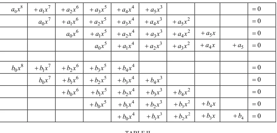
respectively, should be kept constant.Due to these multiplications, the equation (1 a) delivers the next n rows, in the upper part of the matrix, beginning at the left-hand bar of the matrix with the construction of Table I, below, and the equation (1 b) similarly, in the lower part.
Table I, we proposed below, contains the quantities which intervene in the Sylvester procedure for finding common roots or for performing variable elimination between several equations. In this table, cells are filled with terms obtained by the multiplications described above, where the given two equations have been introduced. The multiplication of terms in the case of equations of groups ax and bx, respectively, cease when
(
n−i)
and(
m− j)
, respectively, reach the value zero, and we obtain the terms a5x0 and b4x0.TABLEI
THE TERMS IN THE MATRIX THAT INTERVENE IN THE SYLVESTER METHOD
8 0x
a 7
1x
a
+ 6
2x
a
+ 5
3x
a
+ 4
4x
a
+ 3
5x
a
+ =0
7
0x
a +a1x6 5
2x
a
+ 4
3x
a
+ 3
4x
a
+ 2
5x
a
+ =0
6
0x
a +a1x5 4
2x
a
+ 3
3x
a
+ 2
4x
a
+ +a5x =0
5
0x
a +a1x4 3
2x
a
+ 2
3x
a
+ +a4x +a5 =0
8
0x
b +b1x7 6
2x
b
+ 5
3x
b
+ 4
4x
b
+ =0
7
0x
b +b1x6 5
2x
b
+ 4
3x
b
+ 3
4x
b
+ =0
6
0x
b
+ 5
1x
b
+ 4
2x
b
+ 3
3x
b
+ 2
4x
b
+ =0
5
0x
b
+ 4
1x
b
+ 3
2x
b
+ 2
3x b
+ +b4x =0
4
0x
b
+ 3
1x b
+ 2
2x b
+ +b3x +b4 =0
TABLEII
THE TERMS IN THE DETERMINANT THAT OCCUR IN THE SYLVESTER METHOD
0
a a1 a2 a3 a4 a5
0
a a1 a2 a3 a4 a5
0
a a1 a2 a3 a4 a5
0
a a1 a2 a3 a4 a5
0
b b1 b2 b3 b4
0
b b1 b2 b3 b4
0
b b1 b2 b3 b4
0
b b1 b2 b3 b4
0
[image:2.595.74.524.347.564.2]Therefore, for the cases in which
(
n−i)
and(
m− j)
respectively, become zero, the obtained results will be just the terms of the given polynomials.
In the present case, m=5, n=4.
The free places should be completed with zeroes. There results a matrix and the corresponding determinant with the cells of the main diagonal having non-zero elements, whereas the other cells contain zero as well non-zero elements. The equations above may be considered as a system of m+n equations of the first degree, with m+n unknowns. The right-hand side of every equation, for the adopted arrangement, should be zero.
If, we renounce the straight lines which, in Table I, separate the cells, the remaining symbols, including the addition signs, represent just the equations mentioned above.
If the two equations (1 a, b) have a common root, the quantity x and all its powers (exponents), from 1 to
1 + +n
m , or conversely must fulfil all equations of the system above. The system of equations being compatible, its determinant formed by its coefficients should be zero. A minutely explanation and proof of Sylvester method is given in [3].
In Table I above, the cells are filled with terms obtained by the multiplications also described above, for the two equations. Further on, we shall use only the determinant without the last column of the right-hand side, being not necessary.
It is worth noting that the method may also be deduced from some general remarks. Let us consider two equations of the first degree. For the two equations have a common root, it is necessary their corresponding coefficients be proportional. This condition is equivalent with that the determinant of the system formed by the two equations be zero. Similarly, we can pass to a system formed of three or several equations and unknowns.
Further on, we can replace the unknowns of first degree, by unknowns formed of unknowns at various powers, but so arranged that the power (exponent) does not vary along the same column. Then, every unknown, with any exponent, can represent an unknown having unity as exponent. Thus, we reached the described procedure of Sylvester.
We shall consider an application, namely concerning the two algebraic equations below, written in a form convenient for Maple language (e.g. Maple 12):
( )
x :=x3−17x2+79x−63,F (2 a)
( )
x :=f x3−13x2+44x−32. (2 b)
Further on, we shall write the Sylvester determinant (matrix), and we shall see, taking into account the property of the determinant, if the two equations have or not a common root.
The Sylvester matrix for the chosen example is written below. The matrix for the considered example has been constructed as we explained for Table I, and it will give the needed determinant written in Table III, where the determinant is denoted by C.
TABLEIII
THE MATRIX FOR THE CONSIDERED EXAMPLE
0 −17 79 63− 0 0
0 0 −17 79 63− 0
0 0 0 −17 79 −63
1 −13 44 −32 0 0
0 1 −13 44 −32 0
C=
0 0 1 −13 44 −32
As already mentioned, for the two algebraic equations have a common root, it is necessary and sufficient the determinant of the matrix above be zero. The value of the matrix determinant can easily be calculated by one of the Maple procedures. We chose the following:
with(LinearAlgebra); Determinant
(C, method =rational); (3 a)
with(LinearAlgebra); Determinant
(C, method =float); (3 b)
The two calculation procedures (3 a, b) yield: 0
)
det(C = . (4 a)
− = )
det(C 5.04765174910−12. (4 b)
It is interesting to remark that the matrix method above cannot be considered with the same favourable properties for both aims, namely for finding common roots of a set of polynomials or equations, and for elimination of variables in order to obtain a resultant equation with a smaller number of variables. A difference exists. The reason, may be that in the first case, a single variable x occurs, whereas, for the elimination, even of a single variable between two equations, there can be, at least, two variables.
Another interesting remark emphasized below is that in the case of elimination, other methods can lead to solution even in more difficult cases.
be found, e.g., in the handbook of Maple 12, but we shall present a procedure and results not found in the known literature. The explanations in Maple handbook are there very short. The command eliminate performs the elimination required for certain variables, from a set or list of equations. This elimination is possible for certain given variables. Let us consider an analysis on the next example. For this purpose we shall take the following two equations:
( )
x =x2+y2−a=0F , (5 a)
( )
x =x3−y2x+yx−b=0f . (5 b)
As mentioned, the first step is the determination of a root from one of the two equations. However, it is worth noting that sometimes it is easier to use both equations for this purpose. Multiplying with x both sides of relation (5 a), there follows:
0
2
3+y x−ax=
x . (5 c)
Adding up, side by side, relations (5 b) and (5 c), (namely the parts adjacent to the sign equal), we obtain, after calculation: . 2 ; 2 2
2 y a c y y a
y b
x =− + +
+ + −
= (6)
A. First Procedure
Having now the expression of x deduced from both given equations, for performing the elimination it is necessary and sufficient to introduce this in anyone of the two given equations. We shall introduce it into the first equation (5 a), after separating x2 in the other side of the equation:
( )
x :=F 2 .
2
a y c
b + =
⎟ ⎠ ⎞ ⎜ ⎝ ⎛ (7)
Then, expanding the parenthesis, eliminating the denominator from the right-hand side, and accepting another expression for the left-hand side, hence for
( )
xF ,we get:
( )
x :=F
(
2)
0,expand 2 2 2
2
2 − =
⎟ ⎠ ⎞ ⎜ ⎝ ⎛ − + +
+y y y a ac
b (8 a)
and
( )
x :=F
(
4 3 2 2 2)
2
2 (y a)4y 4y 4y a y 2ya a
b + − − − + + +
. 0 =
(8 b)
It follows, with changed notation, because the denominator has been omitted:
(
)
(
5)
2 .6 1 8 4 4 : 2 3 2 2 2 3 4 5 6 b a a y y a a a y y a y y + − − − + + − − − = Ψ (9)
B. SecondProcedure
We shall introduce now, the expression (6) of x
deduced from both given equations, for performing the elimination, into the second equation (5 b):
( )
=ϕ x : 2 0
3 = − + − ⎟ ⎠ ⎞ ⎜ ⎝
⎛ y x yx b
c b
;
(
2)
03 = − ⎟ ⎠ ⎞ ⎜ ⎝ ⎛ + − + ⎟ ⎠ ⎞ ⎜ ⎝ ⎛ b c b y y c b .
(
2)
2 3 03+ −y +y bc −bc =
b ;
(
2)
2 3 02+ −y +y c −c =
b .
(10 a-d)
After eliminating the denominator and performing the calculations by Maple, and considering a change of the value of ϕ
( )
x , because we omitted the denominator, we get:( )
=ϕ x : b2+
(
−y2+y)
c2−c3=0, (11)( )
=ϕ x :
(
)(
)
(
2)
0,2 3 2 2 2 2 2 = + + − − + + − + − + a y y a y y y y b (12)
(
)
(
5)
2 .6 1 8 4 4 : 2 3 2 2 2 3 4 5 6 b a a y y a a a y y a y y + − − − + + − − − = Ψ (13)
From the results of the applications above, it follows that by the presented procedures for elimination, we obtain for the same case, the same results, even if the calculations differ.
It is interesting to examine if the both procedures studied above, the Sylvester method and the direct methods can be used irrespectively for finding multiple roots of polynomials or for the elimination of certain variables from a set of equations. From the examples above, there follows, that the Sylvester method is rather suitable for finding multiple roots of an algebraic equation or the common roots of a set of equations. Indeed, then, a single variable x once occurs, whereas, for the elimination, even of a single variable, between two equations, there are two variables, say x and y, to be considered.
C. The Calculation by Maple 12
Let us apply the Maple 12 programs. We should emphasize that Table I and Table II cannot be avoided.
D. First Maple Procedure
We shall anew consider the equations above (2 a, b):
( )
x :=x3−17x2+79x−63,F
( )
x :=f x3−13x2+44x−32,
for to establish if they have or not common roots. For this aim, we call in Maple:
with(Algebraic): GreatestCommonDivisor
(
F,f)
Resulting factor is: x−1
Hence the two equations have one common root. The roots are: solve
( )
F, ; result: 1, 7, 9 x( )
f xsolve , ; result: 1, 8, 4
The calculation of the roots has been made by using the Maple programs. Surely, the difficulties for solving each equation remain the well-known. However, the solving of polynomial equations, can be performed regardless of the power (degree) of the equation, even if is greater than four, because Maple allows to use numerical methods, if necessary.
The reason the Maple programs without other completions are not suitable for elimination of certain variables, between two equations, are the same, as mentioned for the Sylvester method, the simultaneous existence of several variables in the same equations. For the case of multiple roots of an equation as well as the case of common roots of a set of equations, the Sylvester procedure with Maple software completions, and the Maple program are equivalent.
There is to be remarked that in the case in which we are looking for the multiple roots of one equation, except the fact that in this case no several equations occur, only the given equation and its derivatives intervene.
E. Second Maple Procedure
Firstly, we come back and start from the preceding equations (5 a, b), with a slight modification, as follows:
. 0 ,
2 3
2 2
= − + −
− =
b y x x y x
y a x
The method which will be presented does not exist in Maple programs or in the known literature, but can be easily prepared by using Maple instructions. From the first equation, we get:
= :
x a−y2 . (14)
Replacing it in equation (5 b), we get:
(
a−y2)
3 −y2(
a−y2) (
+y a−y2)
−b=0. (15)The equation (15) can be rewritten in the form:
(
) (
) ( )
02 2
2 =
− − + − + −
y a
b y
y y
a (16 a)
and
(
) (
)
[
]
22
2 y y
y
a− + − + = 2.
2
y a
b
− (16 b)
After performing and expanding the preceding product, by Maple, there follows:
Expand
(
2 2) (
2 2)
2⎟=0 ⎠ ⎞ ⎜⎝
⎛− − y +y+a ⋅ a−y +b (17)
and the corresponding polynomial, with the chosen sign, will be:
(
)
(
5)
2 .6
1 8 4 4 :
2 3 2 2
2 3
4 5
6
b a a y y a a a y
y a y y
+ − −
− + +
− − − = Ψ
(18)
Hence, the same result as above, by (13), has been obtained.
V. CONCLUSION
We simplified the matrix procedure for the determination of common roots and developed direct methods not found in the known literature, using symbolic programs.
We established that applying the same procedure for obtaining the resultant, after the elimination of certain variables from a set of algebraic equations or polynomials, it is possible to obtain, according to the application manner, different results, but all may be brought to the same form, except when a square root occurs involving the choice of sign.
Therefore, in this case, after performing the elimination, we could have two solution, according to the chosen sign.
Also, we have shown that the direct methods are suitable for elimination of variables (among several equations), whereas the matrix methods are suitable for common roots (of a set of equation) and multiple roots (of a single equation). In all cases, the symbolic language assured much facility.
REFERENCES
[1] E. Knobloch, Determinants and elimination in Leibniz (Déterminants et élimination chez Leibniz), Revue d'histoire des sciences, Volume 54, pp. 143-164 (2001).
[2] R. Zurmühl, S. Falk, Matrizen und ihre Anwendungen. (Matrices and their Applications, Part 2, Numerical methods), Springer Verlag, Berlin, Heidelberg, New York, Tokio, 1986. [3] Ch. de Comberousse, Cours d’Algèbre Supérieure, Seconde Partie, Gauthier-Villars et Fils Imprimeurs-Libraires, Paris, 1890.
Mathematica, vol. XXX, No. 4, 1997, pp. 761-774, Warsaw, Poland.
[5] Th. Anghelutza, Curs de Algebra Superioara (Course of Higher Algebra), Editura Universitatii din Cluj, 1945. [6] G. Strang, The Algebra of Elimination, Massachusetts
Institute of Technology, 2010.
[7] Strang, Introduction to Linear Algebra, Fourth Edition, 1990. [8] P. Stiller, An Introduction to the Theory of Resultants.
Mathematics and Computer Science, T&M University, Texas, College Station, TX.